Local Martingales¶

Run an Itô integral $M_t = \int_0^t \theta_s\,dW_s$ for a wild integrand $\theta$ -- say one whose quadratic variation blows up before some horizon $T$. On every bounded time window the process is driftless: each tiny increment has mean zero. Yet $\mathbb{E}[M_t]$ can still drift below $M_0$, because mass can escape to infinity in the meantime. That gap between local fairness and global fairness is exactly the difference between a local martingale and a true martingale, and it is the failure mode every other page in this section is built to detect and repair (see Unifying Principle).

Mental model

Local martingale = "looks like a fair game locally"
True martingale = "actually fair globally"
Strict local martingale = "appears fair but secretly loses value"

The zero-drift trap

"This process has zero drift, so it's fair." Wrong. Zero drift only gives a local martingale; if it is non-negative, it is actually a supermartingale — so it can still lose value in expectation.

Prerequisites

This section assumes familiarity with:

Definitions¶

Recall that a martingale is an adapted, integrable process satisfying $\mathbb{E}[M_t \mid \mathcal{F}_s] = M_s$ for all $s \leq t$. The local version relaxes this to hold only under stopping.

Local Martingale¶

Local Martingale

An adapted process $\{M_t\}_{t \geq 0}$ with $M_0$ finite almost surely is a local martingale if there exists a sequence of stopping times $\{\tau_n\}_{n=1}^{\infty}$ such that:

Monotonicity: $\tau_1 \leq \tau_2 \leq \tau_3 \leq \cdots$
Divergence: $\tau_n \to \infty$ almost surely as $n \to \infty$
Stopped martingale: The stopped process $M^{\tau_n}_t := M_{t \wedge \tau_n}$ is a martingale for each $n$

The sequence $\{\tau_n\}$ is called a localizing sequence (or reducing sequence).

Remark on condition 3: For $M_{t \wedge \tau_n}$ to be a martingale, we need $\mathbb{E}[|M_{t \wedge \tau_n}|] < \infty$ for all $t$. This is the sense in which localization "tames" potentially non-integrable processes.

Why stopping works

Stopping prevents the process from reaching regions where integrability fails. The localizing sequence "hides the bad behavior" by cutting off the process before extreme events occur. The question is always: can you remove the stopping and still have a martingale?

The Martingale Hierarchy¶

The following inclusions are strict:

\[ \boxed{ \text{UI Martingales} \subsetneq \text{Martingales} \subsetneq \text{Local Martingales} } \]

where UI denotes uniformly integrable. The inclusions go from strongest (UI martingales, the smallest class) to weakest (local martingales, the largest class). A local martingale that is not a true martingale is called a strict local martingale.

Connection to Convergence Theory

Uniformly integrable martingales converge in $L^1$, not just almost surely. See Martingale Convergence for the full hierarchy of convergence results.

What Can Go Wrong?¶

A local martingale fails to be a true martingale for two fundamentally different reasons.

1. Integrability Failure¶

The process is not even a martingale candidate:

\[ \mathbb{E}[|M_t|] = \infty \quad \text{for some } t > 0 \]

2. Integrability Holds, but Martingale Property Fails¶

Even when $\mathbb{E}[|M_t|] < \infty$, the martingale property can fail because limits do not commute with expectation. When we localize and take $n \to \infty$, Fatou's lemma only gives an inequality — and the direction of that inequality depends on the sign of $M$.

The direction of failure is determined by the sign of $M$:

(a) If $M_t \geq 0$ (non-negative local martingale). Let $\{\tau_n\}$ be a localizing sequence. Each stopped process $M_{t \wedge \tau_n}$ is a true martingale, so:

\[ \mathbb{E}[M_{t \wedge \tau_n}] = \mathbb{E}[M_0] \quad \text{for every } n \]

Since $M_{t \wedge \tau_n} \to M_t$ a.s. (as $\tau_n \uparrow \infty$) and $M_{t \wedge \tau_n} \geq 0$, Fatou's lemma applies:

\[ \mathbb{E}[M_t] = \mathbb{E}\!\left[\liminf_{n \to \infty} M_{t \wedge \tau_n}\right] \leq \liminf_{n \to \infty} \mathbb{E}[M_{t \wedge \tau_n}] = \mathbb{E}[M_0] \]

Equality makes $M$ a true martingale; strict inequality signals mass loss at infinity.

Why the inequality can be strict. Upgrading $\leq$ to $=$ would require interchanging limit and expectation, which needs uniform integrability or dominated convergence. When neither holds, the mechanism is:

At each finite $n$, the stopping time $\tau_n$ cuts off the process before extreme values are reached, so $\mathbb{E}[M_{t \wedge \tau_n}] = M_0$ holds exactly.
As $n$ increases, $\tau_n$ lets the process run longer — rare paths where $M_t$ becomes very large are cut off later and later.
Although these extreme paths are rare, they carry large values and contribute disproportionately to the expectation.
In the limit $n \to \infty$, these paths are never cut, but their contribution to the expectation does not come back nicely — it is lost in the passage from $\liminf$ of expectations to expectation of $\liminf$.

\[ \boxed{\text{Stopping preserves fairness, but removing the stopping lets rare large values escape — Fatou turns equality into inequality.}} \]

Toy model: rare spikes that pointwise limits miss

Define $X_n = n \cdot \mathbf{1}_{\{U \leq 1/n\}}$ where $U \sim \text{Uniform}(0,1)$.

Each $X_n$ has expectation 1: $\mathbb{E}[X_n] = n \cdot \tfrac{1}{n} = 1$.
Pointwise limit is 0: for any fixed $u > 0$, eventually $u > 1/n$, so $X_n(u) = 0$.
Fatou gap: $\mathbb{E}[\liminf X_n] = 0 < 1 = \liminf \mathbb{E}[X_n]$.

The spike at each stage is rare (probability $1/n$) but large (size $n$), so it sustains the expectation. But no single sample path ever sees a spike in the limit — the mass escapes through ever-rarer events. This is exactly the mechanism behind strict local martingales: expectation sees rare huge values; pointwise limits do not.

Signed contrast: the doubling strategy

A gambler bets $\$2^{n-1}$ on round $n$ until the first head at time $T = \inf\{n \geq 1 : \text{toss } n \text{ is Head}\}$. The cumulative wealth is:

\[ S_n = \mathbf{1}_{\{T \leq n\}} - (2^n - 1)\,\mathbf{1}_{\{T > n\}} \]

Then $\mathbb{E}[S_n] = (1 - 2^{-n}) - (2^n - 1) \cdot 2^{-n} = 0$ for every $n$ (fair game), but $S_n \to 1$ a.s. since $T < \infty$ a.s. So:

\[ \mathbb{E}[\lim S_n] = 1 > 0 = \lim \mathbb{E}[S_n] \]

Here the rare negative tail (catastrophic loss $-(2^n - 1)$ with probability $2^{-n}$) disappears pathwise, so the limit expectation is larger. In a non-negative strict local martingale, the rare positive tail disappears instead, so the limit expectation is smaller. The mechanism is the same — compensating mass hides in rarer and rarer extreme events — but the sign determines the direction.

(b) If $M_t \leq 0$ (non-positive local martingale). Apply Fatou to $-M$:

\[ \mathbb{E}[M_t] \geq \mathbb{E}[M_0] \]

Equality makes $M$ a true martingale; strict inequality signals mass gain from $-\infty$ (sign-flipped leakage).

(c) No Sign Constraint (General Case). If $M$ has no sign restriction, then no inequality is forced by Fatou alone — $\mathbb{E}[M_t]$ can lie above or below $\mathbb{E}[M_0]$. The outcome depends on which tail dominates: large positive excursions push the expectation down, while large negative excursions push it up.

One-line summary

A local martingale fails either because it is not integrable, or because localization hides tail behavior, and the direction of failure is dictated by the sign via Fatou.

Canonical Examples¶

Example 1: Itô Integrals¶

Consider the Itô integral:

\[ M_t = \int_0^t \sigma_s\,dW_s \]

where $\sigma$ is an adapted process.

Integrability Hierarchy for Itô Integrals

Condition	Result
$\int_0^t \sigma_s^2 \, ds < \infty$ a.s.	Integral exists; local martingale
$\mathbb{E}\left[\int_0^T \sigma_s^2 \, ds\right] < \infty$	True martingale on $[0,T]$
Neither	Integral not defined

The a.s. condition is the existence requirement—without it, the Itô integral is not even defined. The $L^1$ condition upgrades local martingale to true martingale.

Intuition: A driftless SDE $dM_t = \sigma_t dW_t$ looks like a martingale—it's "pure noise" with no systematic drift. And usually it is a true martingale. But technically, Itô calculus only guarantees a local martingale; upgrading to true martingale requires verifying integrability.

Proof that it's a local martingale: Define the localizing sequence:

\[ \tau_n = \inf\left\{t \geq 0 : \int_0^t \sigma_s^2\,ds \geq n\right\} \wedge n \]

Then $\tau_n \uparrow \infty$ a.s., and by construction:

\[ \mathbb{E}\left[\int_0^{T \wedge \tau_n} \sigma_s^2\,ds\right] \leq n < \infty \]

By the Itô isometry criterion, $M_{t \wedge \tau_n}$ is a true martingale for each $n$. $\square$

Pattern recognition

Driftless SDE → always a local martingale. Then check $L^2$ (Itô isometry) to upgrade.

Example 2: Stochastic Exponential (True Martingale)¶

Recall (see § The Stochastic Exponential): $\mathcal{E}(W)_t = \exp(W_t - t/2)$ solves $dZ_t = Z_t\,dW_t$ with $Z_0 = 1$, so it is always a local martingale.

Claim: $\mathcal{E}(W)_t$ is a true martingale with $\mathbb{E}[\mathcal{E}(W)_t] = 1$ for all $t \geq 0$.

Proof: Here $\langle W \rangle_t = t$ is deterministic, so $\mathbb{E}[\exp(\frac{1}{2}\langle W \rangle_T)] = e^{T/2} < \infty$. By Novikov's theorem (see § Novikov and Kazamaki Conditions), $\mathcal{E}(W)$ is a true martingale. $\square$

Pattern recognition

Stochastic exponential = candidate density for measure change. Always a local martingale — needs Novikov to be valid.

Example 3: Reciprocal of 3D Bessel Process (Strict Local Martingale)¶

Let $R_t = |B_t|$ where $B_t = (B^1_t, B^2_t, B^3_t)$ is 3-dimensional Brownian motion started from $B_0 = x$ with $|x| = r_0 > 0$. The process $R_t$ is the 3-dimensional Bessel process started from $r_0$.

Define:

\[ M_t = \frac{1}{R_t} \]

Claim: $M_t$ is a strict local martingale (local martingale but NOT a true martingale).

Common Misconception

The failure is not because $R_t$ hits zero. In fact, the 3D Bessel process is transient: $R_t \to \infty$ as $t \to \infty$ almost surely, and $R_t > 0$ for all $t \geq 0$ when $r_0 > 0$.

Proof that $M_t$ is a local martingale:

The $d$-dimensional Bessel process satisfies the SDE:

\[ dR_t = \frac{d-1}{2R_t}dt + dW_t \]

where $W$ is a 1-dimensional Brownian motion. For $d = 3$, this gives $dR_t = \frac{1}{R_t}dt + dW_t$.

By Itô's formula applied to $f(r) = 1/r$:

\[ d\left(\frac{1}{R_t}\right) = -\frac{1}{R_t^2}dR_t + \frac{1}{R_t^3}dt = -\frac{1}{R_t^2}\left(\frac{1}{R_t}dt + dW_t\right) + \frac{1}{R_t^3}dt = -\frac{1}{R_t^2}dW_t \]

The drift terms cancel! Thus $M_t = 1/R_t$ satisfies:

\[ dM_t = -\frac{1}{R_t^2}dW_t \]

This is an Itô integral (no drift), hence a local martingale.

Proof that $M_t$ is NOT a true martingale:

Using the transition density of the 3D Bessel process (see Revuz–Yor, Chapter VI, or Karatzas–Shreve §3.3.C), one can compute:

\[ \mathbb{E}\left[\frac{1}{R_t}\right] = \frac{1}{r_0} - \frac{2}{r_0}\Phi\left(-\frac{r_0}{\sqrt{t}}\right) < \frac{1}{r_0} = M_0 \]

where $\Phi$ is the standard normal CDF. The strict inequality shows $\mathbb{E}[M_t] < \mathbb{E}[M_0]$, violating the martingale property.

Intuition: As $t \to \infty$, the Bessel process drifts to $+\infty$, so $1/R_t \to 0$. The "probability mass" that would be needed to maintain $\mathbb{E}[M_t] = M_0$ has "leaked to infinity."

Pattern recognition

This is the canonical "strict local martingale without explosion" example. The paths remain finite, yet expectation drops — mass leakage, not blow-up.

Example 4: CEV Model with β > 1 (Strict Local Martingale)¶

The constant elasticity of variance (CEV) model provides a clean example of a strict local martingale arising in finance. Consider:

\[ dX_t = \sigma X_t^\beta \, dW_t, \quad X_0 = x_0 > 0 \]

where $\sigma > 0$ and $\beta > 1$.

Claim: For $\beta > 1$, the process $X_t$ is a strict local martingale.

Why this is a local martingale: The process is clearly a local martingale since it is an Itô integral with no drift term. The localizing sequence:

\[ \tau_n = \inf\{t \geq 0 : X_t \geq n \text{ or } X_t \leq 1/n\} \wedge n \]

ensures $X_{t \wedge \tau_n}$ is bounded and hence a true martingale.

Why this is NOT a true martingale: For $\beta > 1$, boundary classification shows that the process exhibits strict local martingale behavior: $\mathbb{E}[X_t] < X_0$ for all $t > 0$. The failure is not best understood as simple pathwise explosion, but rather as a failure of integrability sufficient to preserve expectation — mass escapes to infinity in expectation.

\[ \mathbb{E}[X_t] < x_0 \quad \text{for all } t > 0 \]

Financial interpretation: The CEV model with $\beta > 1$ exhibits explosive behavior inconsistent with limited liability. This is why practitioners typically use $\beta < 1$ (which gives absorption at zero rather than explosion at infinity).

Pattern recognition

Volatility that increases with price ($\sigma X^\beta$, $\beta > 1$) pushes probability mass outward, causing expectation to drop. Bubbles can arise from volatility structure and boundary behavior, not just drift.

Mathematical Characterization¶

The Supermartingale Property¶

Key insight

Non-negative local martingales can only lose expectation, never gain it. If $\mathbb{E}[M_t] < \mathbb{E}[M_0]$, immediately think: strict local martingale.

Non-negative Local Martingales are Supermartingales

Let $M$ be a non-negative local martingale. Then $M$ is a supermartingale:

\[ \mathbb{E}[M_t \mid \mathcal{F}_s] \leq M_s \quad \text{almost surely for all } 0 \leq s \leq t \]

Proof: Apply the Fatou argument from What Can Go Wrong? with conditional rather than unconditional expectations: $\mathbb{E}[M_t \mid \mathcal{F}_s] \leq \liminf_n \mathbb{E}[M_{t \wedge \tau_n} \mid \mathcal{F}_s] = \liminf_n M_{s \wedge \tau_n} = M_s$. $\square$

Corollary: For non-negative local martingales:

\[ \mathbb{E}[M_t] \leq \mathbb{E}[M_0] \]

with equality if and only if $M$ is a true martingale.

Sufficient Conditions for True Martingale¶

Recall (see § Integrability Conditions for Martingales): every sufficient criterion works by ruling out mass leakage, ultimately via uniform integrability. In brief:

Boundedness, domination, $L^p$ boundedness ($p > 1$), or finite expected quadratic variation (BDG) — see § Integrability Conditions for Martingales
Novikov or Kazamaki for stochastic exponentials — see § Novikov and Kazamaki Conditions

Connection to Infinitesimal Generators¶

Let $X_t$ be a diffusion with infinitesimal generator:

\[ \mathcal{L} = \mu(x)\frac{\partial}{\partial x} + \frac{1}{2}\sigma^2(x)\frac{\partial^2}{\partial x^2} \]

For $f \in C^2$, define the process $Y_t = f(X_t)$.

Generator Criterion

If $\mathcal{L}f(x) = 0$ for all $x$ in the state space, then $f(X_t)$ is a local martingale.

To upgrade to a true martingale, verify any of the sufficient conditions above (boundedness, domination, $L^p$ bounds, finite quadratic variation, or Novikov/Kazamaki for stochastic exponentials).

Connection to Dynkin's formula: By Itô's formula:

\[ f(X_t) - f(X_0) = \int_0^t \mathcal{L}f(X_s)\,ds + \int_0^t f'(X_s)\sigma(X_s)\,dW_s \]

When $\mathcal{L}f = 0$, the drift integral vanishes, leaving only the stochastic integral (which is a local martingale).

See Generator and Martingales for the full treatment.

Financial Implications¶

Math	Finance
Local martingale	Candidate price process
True martingale	Valid pricing (expectations preserved)
Strict local martingale	Bubble (market price exceeds fundamental value)

Discounted Asset Prices¶

The discounted asset price is defined as:

\[ \tilde{S}_t = e^{-rt}S_t \]

Under the risk-neutral measure $\mathbb{Q}$, the discounted asset price is required to be a local martingale for the market to satisfy the no-arbitrage condition (in the sense of NFLVR). In many models, one further verifies that it is a true martingale, which ensures well-behaved pricing via expectations.

In practice, $\tilde{S}_t$ is often only a local martingale. The distinction matters.

Strict Local Martingales and Financial Bubbles¶

Bubble Characterization

If the discounted price process is a strict local martingale under $\mathbb{Q}$:

\[ \mathbb{E}^{\mathbb{Q}}[e^{-rT}S_T] < S_0 \]

This implies the current price $S_0$ exceeds its "fundamental value" (the discounted expected future price). This is the mathematical signature of a financial bubble.

Reference: Jarrow, Protter, and Shimbo (2010), "Asset Price Bubbles in Incomplete Markets," Mathematical Finance.

Put-Call Parity Failure¶

The standard put-call parity:

\[ C(K,T) - P(K,T) = S_0 - Ke^{-rT} \]

relies on $\mathbb{E}^{\mathbb{Q}}[e^{-rT}S_T] = S_0$. When the stock price is a strict local martingale:

\[ C(K,T) - P(K,T) = \mathbb{E}^{\mathbb{Q}}[e^{-rT}S_T] - Ke^{-rT} < S_0 - Ke^{-rT} \]

Put-call parity fails, and the put price includes a "bubble premium."

Connection to Girsanov's Theorem¶

Recall (see § Girsanov's Theorem): the Girsanov density $Z_t = \mathcal{E}(-\int_0^\cdot \theta_s\,dW_s)_t$ must be a true martingale (not merely local) — this is where Novikov / Kazamaki enter.

Summary Table¶

Property	Martingale	Local Martingale	Strict Local Martingale
Definition	$\mathbb{E}[M_t \mid \mathcal{F}_s] = M_s$	$M_{t\wedge\tau_n}$ is martingale	Local mart., not true mart.
Integrability	Required: $\mathbb{E}[	M_t	] < \infty$
Mean preservation	$\mathbb{E}[M_t] = \mathbb{E}[M_0]$	$\mathbb{E}[M_t] \leq \mathbb{E}[M_0]$	$\mathbb{E}[M_t] < \mathbb{E}[M_0]$
If $M \geq 0$	Supermartingale	Supermartingale	Strict supermartingale
Explosion	Cannot explode	Can explode	May or may not explode
Financial interpretation	Fair game	Locally fair	Bubble possible

Key Takeaways¶

\[ \boxed{ \mathcal{L}f = 0 \implies f(X_t) \text{ is a local martingale} } \]

\[ \boxed{ \mathcal{L}f = 0 \text{ + sufficient condition} \implies f(X_t) \text{ is a true martingale} } \]

\[ \boxed{ \text{Non-negative local martingale} \implies \text{Supermartingale} } \]

\[ \boxed{ \mathbb{E}[M_t] < \mathbb{E}[M_0] \text{ for non-negative } M \iff M \text{ is a strict local martingale} } \]

The Bottom Line

The distinction between local martingales and true martingales is essential for:

Rigorous Itô calculus: Ensuring stochastic integrals have the expected properties
Measure changes: Validating Girsanov transformations via Novikov/Kazamaki
Financial modeling: Detecting and modeling asset price bubbles
PDE connections: Understanding when Feynman–Kac representations hold

Python Simulation: Mass Leakage in Strict Local Martingales¶

The following simulation demonstrates how $\mathbb{E}[M_t]$ can decrease over time for a strict local martingale.

```python import numpy as np import matplotlib.pyplot as plt

def simulate_inverse_bessel_3d(r0, T, dt, n_paths): """ Simulate 1/R_t where R_t is a 3D Bessel process. This is a strict local martingale. """ n_steps = int(T / dt) t = np.linspace(0, T, n_steps + 1)

# Simulate 3D Brownian motion
dW = np.sqrt(dt) * np.random.randn(n_paths, n_steps, 3)
B = np.zeros((n_paths, n_steps + 1, 3))
B[:, 0, :] = r0 / np.sqrt(3)  # Start at distance r0 from origin

for i in range(n_steps):
    B[:, i+1, :] = B[:, i, :] + dW[:, i, :]

# Compute R_t = |B_t|
R = np.sqrt(np.sum(B**2, axis=2))
R = np.maximum(R, 1e-10)  # Avoid division by zero

# M_t = 1/R_t
M = 1.0 / R

return t, M, R

Parameters¶

r0 = 1.0 T = 5.0 dt = 0.001 n_paths = 50000

np.random.seed(42) t, M, R = simulate_inverse_bessel_3d(r0, T, dt, n_paths)

Compute E[M_t] over time¶

E_M = np.mean(M, axis=0)

Theoretical initial value¶

M0 = 1.0 / r0

Plot¶

fig, axes = plt.subplots(1, 2, figsize=(14, 5))

Left: E[M_t] over time¶

ax1 = axes[0] ax1.plot(t, E_M, 'b-', linewidth=2, label=r'$\mathbb{E}[M_t]$ (Monte Carlo)') ax1.axhline(y=M0, color='r', linestyle='--', linewidth=2, label=r'$M_0 = 1/r_0$') ax1.set_xlabel('Time $t$', fontsize=12) ax1.set_ylabel(r'$\mathbb{E}[M_t]$', fontsize=12) ax1.set_title('Mass Leakage in Strict Local Martingale\n(Inverse 3D Bessel Process)', fontsize=12) ax1.legend(fontsize=11) ax1.grid(True, alpha=0.3) ax1.set_ylim([0, M0 * 1.1])

Right: Sample paths¶

ax2 = axes[1] n_show = 20 for i in range(n_show): ax2.plot(t, M[i, :], alpha=0.5, linewidth=0.5) ax2.set_xlabel('Time $t$', fontsize=12) ax2.set_ylabel(r'$M_t = 1/R_t$', fontsize=12) ax2.set_title(f'Sample Paths ({n_show} shown)', fontsize=12) ax2.grid(True, alpha=0.3) ax2.set_ylim([0, 5])

plt.tight_layout() plt.savefig('strict_local_martingale_simulation.png', dpi=150, bbox_inches='tight') plt.show()

Print summary statistics¶

print(f"Initial value M_0 = 1/r_0 = {M0:.4f}") print(f"E[M_T] at T={T}: {E_M[-1]:.4f}") print(f"Mass leakage: {(M0 - E_M[-1])/M0 * 100:.2f}%") ```

Output:

Initial value M_0 = 1/r_0 = 1.0000 E[M_T] at T=5.0: 0.3471 Mass leakage: 65.29%

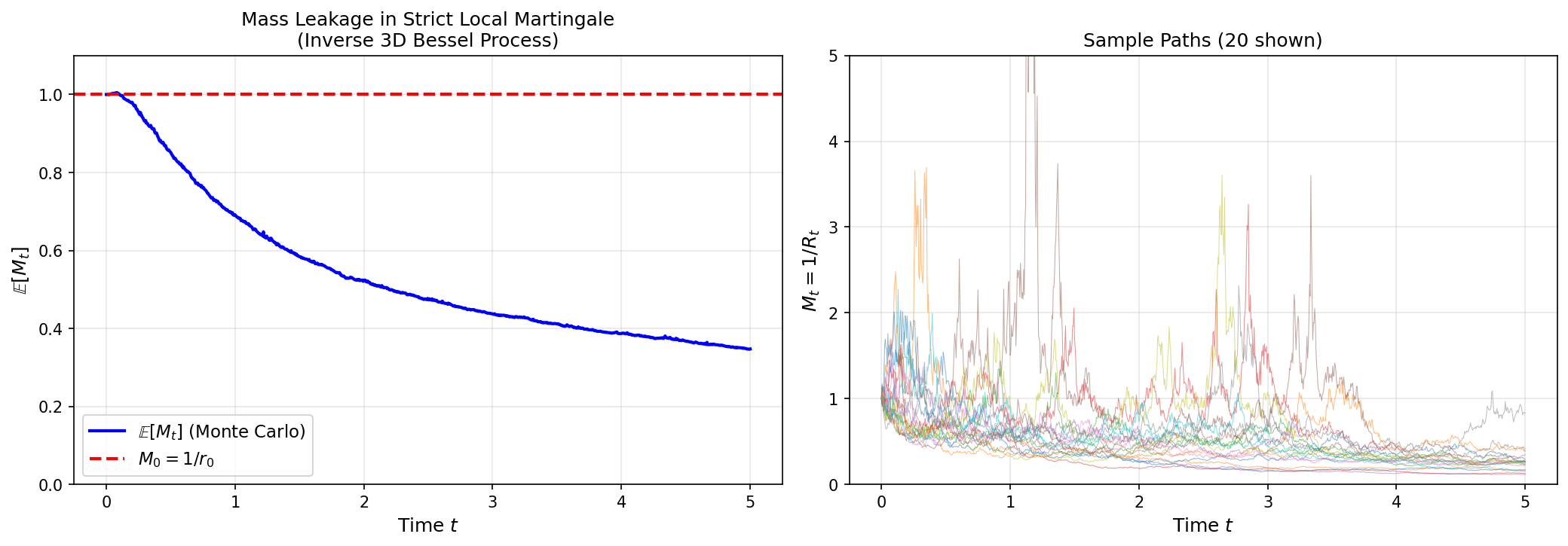
Strict Local Martingale Simulation

Interpretation: The plot shows $\mathbb{E}[M_t]$ decreasing below $M_0 = 1$, demonstrating the strict local martingale property. The "leaked mass" corresponds to paths where $R_t$ has drifted far from the origin—as the 3D Bessel process is transient and escapes to infinity, $1/R_t \to 0$, but the expectation cannot be preserved because the probability mass needed to compensate has "escaped to infinity."

Exercises¶

Exercise 1. Prove that every true martingale is a local martingale. Then explain why the converse fails by giving the key property that a strict local martingale violates.

Solution to Exercise 1

Every true martingale is a local martingale: Let $M_t$ be a true martingale. Define $\tau_n = n$ for all $n \geq 1$. Then $\tau_n \to \infty$, and $M_{t \wedge \tau_n} = M_{t \wedge n}$ is a martingale (a stopped martingale is still a martingale). Hence $M$ is a local martingale with localizing sequence $\{\tau_n = n\}$.

The converse fails: A strict local martingale can fail to be a true martingale in two ways. First, integrability itself may fail: $\mathbb{E}[|M_t|] = \infty$ for some $t$. Second — and more subtly — integrability may hold ($\mathbb{E}[|M_t|] < \infty$) while the martingale property still fails because Fatou's lemma only gives an inequality when passing from stopped to unstopped processes. For a non-negative strict local martingale this means $\mathbb{E}[M_t \mid \mathcal{F}_s] \leq M_s$ (supermartingale, not martingale) and $\mathbb{E}[M_t] < \mathbb{E}[M_0]$ — the expectation strictly decreases over time because large values escape integrably at each localization step.

Exercise 2. You simulate a non-negative process and observe that:

sample paths look symmetric,
no visible drift,
but the empirical mean decreases over time.

What is the most likely explanation? Why can a process appear driftless pathwise yet lose expectation globally?

Solution to Exercise 2

The process is most likely a strict local martingale. Pathwise it looks driftless — each stopped version is a true martingale — but globally the mean falls because rare, large tail events break the martingale equality.

The mechanism is as follows. At each localization level $\tau_n$, the stopped process $M_{t \wedge \tau_n}$ is a true martingale with $\mathbb{E}[M_{t \wedge \tau_n}] = M_0$. As $n \to \infty$, the stopping lets the process run longer, exposing rare paths where $M_t$ takes very large values. These extreme paths are too rare to affect typical sample paths (so the simulation looks symmetric), but they carry enough mass to sustain the expectation. When the stopping is fully removed, Fatou's lemma only gives $\mathbb{E}[M_t] \leq M_0$ — the mass carried by these rare paths "escapes to infinity" and the expectation drops.

This is why "no visible drift" does not imply martingale: the simulation shows typical paths, but the mean is governed by rare extremes that no finite sample captures faithfully.

Exercise 3. Recall from Example 3 that the process $M_t = 1/R_t$ satisfies $dM_t = -M_t^2\,dW_t$ — zero drift, pure noise. Yet it is not a true martingale. Explain precisely which assumption of the martingale definition fails, and why simulations would not reveal the failure.

Solution to Exercise 3

From Example 3, $M_t = 1/R_t$ satisfies

\[ dM_t = -M_t^2\,dW_t. \]

There is no $dt$ term, so the process has zero drift in differential form. Pathwise it looks like pure noise.

However, $M_t$ is not a true martingale. It is a strict local martingale, because $\mathbb{E}[M_t] < M_0$.

The issue is not the formal martingale identity after stopping; each localized process is a true martingale. What fails globally is the step from local martingale to true martingale: one cannot justify passing from the stopped martingale identities to the unstopped process without extra integrability or uniform integrability. The failed assumption is the global martingale requirement $\mathbb{E}[M_t \mid \mathcal{F}_s] = M_s$.

Why simulations can mislead. Typical simulated paths show ordinary fluctuations. The failure comes from rare tail events that affect expectation but are hard to see in finite samples. A Monte Carlo estimate of $\mathbb{E}[M_t]$ will eventually show a declining mean (see Exercise 9), but individual paths give no hint of trouble.

Exercise 4. Let $M_t$ be a non-negative local martingale with $M_0 = 1$. Using Fatou's lemma, prove the supermartingale inequality $\mathbb{E}[M_t] \leq 1$ for all $t \geq 0$. Explain the financial interpretation of $1 - \mathbb{E}[M_t]$ when $M_t$ is the discounted price of an asset under the risk-neutral measure.

Solution to Exercise 4

Let $M_t$ be a non-negative local martingale with $M_0 = 1$ and localizing sequence $\{\tau_n\}$. For each $n$, $M_{t \wedge \tau_n}$ is a true martingale, so:

\[ \mathbb{E}[M_{t \wedge \tau_n}] = \mathbb{E}[M_0] = 1 \]

As $n \to \infty$, $\tau_n \to \infty$ a.s., so $M_{t \wedge \tau_n} \to M_t$ a.s. Since $M_t \geq 0$, Fatou's lemma gives:

\[ \mathbb{E}[M_t] = \mathbb{E}\left[\liminf_{n \to \infty} M_{t \wedge \tau_n}\right] \leq \liminf_{n \to \infty} \mathbb{E}[M_{t \wedge \tau_n}] = 1 \]

Financial interpretation: When $M_t$ is the discounted price of an asset under $\mathbb{Q}$, the quantity $1 - \mathbb{E}[M_t]$ represents the bubble component. If $M_t$ is a strict local martingale, $\mathbb{E}[M_t] < 1 = M_0$, meaning the current asset price exceeds its "fundamental value" $\mathbb{E}^{\mathbb{Q}}[e^{-rT}S_T]$ by the amount $S_0(1 - \mathbb{E}[M_t])$. This excess is the mathematical signature of a financial bubble.

Exercise 5. Let $M_t$ be a local martingale.

(a) If $M_t \geq 0$, show that $\mathbb{E}[M_t] \leq \mathbb{E}[M_0]$.

(b) If $M_t \leq 0$, show that $\mathbb{E}[M_t] \geq \mathbb{E}[M_0]$.

Explain intuitively why the direction of inequality depends on the sign.

Solution to Exercise 5

Let $\{\tau_n\}$ be a localizing sequence. Then for each $n$, the stopped process $M_{t \wedge \tau_n}$ is a true martingale, so

\[ \mathbb{E}[M_{t \wedge \tau_n}] = \mathbb{E}[M_0]. \]

(a) Non-negative case. Suppose $M_t \geq 0$. Since $M_{t \wedge \tau_n} \to M_t$ a.s. and the stopped variables are non-negative, Fatou's lemma gives

\[ \mathbb{E}[M_t] = \mathbb{E}\!\left[\liminf_{n\to\infty} M_{t \wedge \tau_n}\right] \leq \liminf_{n\to\infty}\mathbb{E}[M_{t \wedge \tau_n}] = \mathbb{E}[M_0]. \]

(b) Non-positive case. Suppose $M_t \leq 0$. Then $-M_t \geq 0$, and $-M$ is also a local martingale. Applying part (a) to $-M$:

\[ \mathbb{E}[-M_t] \leq \mathbb{E}[-M_0]. \]

Multiplying by $-1$ reverses the inequality:

\[ \mathbb{E}[M_t] \geq \mathbb{E}[M_0]. \]

Intuition. Fatou's lemma naturally controls non-negative quantities. If the process is non-negative, rare large positive excursions can disappear in the limit and expectation can only go down. If the process is non-positive, apply the same logic to $-M$: now rare large negative excursions disappear, so the expectation of $M$ goes up. The sign determines which tail can "leak away," and therefore determines the direction of the inequality.

Exercise 6. Let $M_t$ be a non-negative local martingale with $M_0 = 1$. You observe that $\mathbb{E}[M_t] < M_0$ for some $t > 0$. Which of the following must be true?

(A) Arbitrage exists.

(B) The model is wrong.

(C) $M_t$ is a strict local martingale.

(D) Cannot conclude.

Justify your answer.

Solution to Exercise 6

The answer is (C).

Since $M_t \geq 0$ and is a local martingale, it is automatically a supermartingale, so $\mathbb{E}[M_t] \leq M_0$. Furthermore, equality $\mathbb{E}[M_t] = M_0$ holds if and only if $M_t$ is a true martingale. Therefore, the strict inequality $\mathbb{E}[M_t] < M_0$ is exactly the defining signature of a strict local martingale.

Why the other choices fail:

(A) A strict local martingale does not by itself imply arbitrage. Strict local martingales are consistent with NFLVR (no free lunch with vanishing risk); what fails is the classical no-arbitrage pricing formula, not the absence of arbitrage strategies.
(B) The observation is perfectly consistent with a well-specified model — strict local martingales arise naturally (e.g., inverse 3D Bessel process, CEV with $\beta > 1$).
(D) We can conclude: for a non-negative local martingale, $\mathbb{E}[M_t] < M_0$ is equivalent to $M_t$ being a strict local martingale.

Financial interpretation. If $M_t$ is the discounted asset price under the risk-neutral measure, the gap $M_0 - \mathbb{E}[M_t] > 0$ is the bubble component: the current price exceeds the discounted expected future payoff. The market is not mispriced in the arbitrage sense — no riskless profit is available — but the price contains a speculative premium that will vanish over time as $\mathbb{E}[M_t]$ drifts below $M_0$.

Exercise 7. Let $M_t$ be a local martingale and suppose the family $\{M_{t \wedge \tau_n}\}_n$ is uniformly integrable for each fixed $t$. Show that $M_t$ is a true martingale.

Solution to Exercise 7

Fix $0 \leq s \leq t$. For each $n$,

\[ \mathbb{E}[M_{t \wedge \tau_n} \mid \mathcal{F}_s] = M_{s \wedge \tau_n}. \]

Since $\tau_n \uparrow \infty$ a.s., we have $M_{t \wedge \tau_n} \to M_t$ and $M_{s \wedge \tau_n} \to M_s$ a.s.

Since $\{M_{t \wedge \tau_n}\}_n$ is uniformly integrable and converges a.s., it converges in $L^1$. Therefore

\[ \mathbb{E}[M_{t \wedge \tau_n} \mid \mathcal{F}_s] \to \mathbb{E}[M_t \mid \mathcal{F}_s] \quad \text{in } L^1. \]

But for each $n$, $\mathbb{E}[M_{t \wedge \tau_n} \mid \mathcal{F}_s] = M_{s \wedge \tau_n}$. Taking limits:

\[ \mathbb{E}[M_t \mid \mathcal{F}_s] = \lim_{n\to\infty} M_{s \wedge \tau_n} = M_s. \]

Also, $L^1$ convergence implies $M_t \in L^1$, so integrability holds. Therefore $M$ is a true martingale.

Key idea. For a non-negative local martingale, localization plus Fatou gives only the supermartingale inequality $\mathbb{E}[M_t \mid \mathcal{F}_s] \leq M_s$. Uniform integrability is what restores equality: since $M_{t \wedge \tau_n} \to M_t$ in $L^1$, conditional expectations also converge in $L^1$, so the martingale identity survives the limit.

Exercise 8. Let $M_t = \int_0^t \sigma_s\,dW_s$ where $\sigma_s = 1/(1 - s)$ for $s \in [0, 1)$. Show that $\int_0^1 \sigma_s^2\,ds = +\infty$ but $\int_0^t \sigma_s^2\,ds < \infty$ for every $t < 1$. Construct a localizing sequence $\{\tau_n\}$ that makes $M_{t \wedge \tau_n}$ a true martingale for each $n$, and explain how localization hides the failure of global integrability near the terminal time $t = 1$.

Solution to Exercise 8

We have $\sigma_s = 1/(1-s)$ for $s \in [0,1)$. For $t < 1$:

\[ \int_0^t \sigma_s^2\,ds = \int_0^t \frac{1}{(1-s)^2}\,ds = \left[\frac{1}{1-s}\right]_0^t = \frac{1}{1-t} - 1 = \frac{t}{1-t} < \infty \]

As $t \to 1^-$, this diverges: $\int_0^1 \sigma_s^2\,ds = \lim_{t \to 1^-} \frac{t}{1-t} = +\infty$.

For the localizing sequence, define:

\[ \tau_n = \inf\left\{t \geq 0 : \int_0^t \sigma_s^2\,ds \geq n\right\} \wedge \left(1 - \frac{1}{n}\right) \]

Then $\tau_n \uparrow 1$ a.s. as $n \to \infty$, and by construction:

\[ \int_0^{T \wedge \tau_n} \sigma_s^2\,ds \leq n < \infty \]

Since $\mathbb{E}\left[\int_0^{T \wedge \tau_n} \sigma_s^2\,ds\right] \leq n < \infty$, the Itô isometry criterion guarantees that $M_{t \wedge \tau_n} = \int_0^{t \wedge \tau_n} \sigma_s\,dW_s$ is a true (square-integrable) martingale for each $n$.

How localization hides the failure. At the terminal time $t = 1$, the quadratic variation $\int_0^1 \sigma_s^2\,ds$ diverges, so the stochastic integral is no longer defined as an $L^2$ object. The process cannot satisfy the integrability requirement $\mathbb{E}[|M_t|] < \infty$ for a true martingale. Localization hides this pathology by cutting off the process before the variance explodes: each $\tau_n$ stops the process early enough that the stopped integral remains square-integrable, preserving the martingale property up to time $\tau_n$.

Exercise 9. You are given two non-negative processes, both starting at $M_0 = 1$:

Process A is a true martingale.
Process B is a strict local martingale.

Both look identical over short time scales. How would you statistically distinguish them using Monte Carlo simulation?

Solution to Exercise 9

Track the empirical mean $\bar{M}_t = \frac{1}{N}\sum_{i=1}^N M_t^{(i)}$ across many independent paths as a function of time $t$:

Process A (true martingale): $\bar{M}_t \approx M_0 = 1$ for all $t$. The empirical mean stays flat.
Process B (strict local martingale): $\bar{M}_t$ decreases below $M_0$ as $t$ grows, because $\mathbb{E}[M_t] < M_0$.

The key diagnostic is therefore the time profile of the sample mean. A declining empirical mean signals a strict local martingale.

A subtlety: with a finite number of paths $N$, the rare large values that sustain the stopped expectation may occasionally appear in the sample, causing the empirical mean to jump erratically. As $t$ increases these extreme events become rarer, so the sample mean settles below $M_0$. Increasing both $N$ and $t$ makes the distinction sharper.

Exercise 10. Consider the CEV model $dX_t = \sigma X_t^{\beta}\,dW_t$ with $X_0 = 1$ and $\sigma = 0.5$. For $\beta = 0.5$, verify that $X_t$ is a true martingale by checking that $\mathbb{E}[\langle X \rangle_T] < \infty$. For $\beta = 1.5$, explain heuristically — using the discussion of strict local martingales in this section — why $X_t$ is only a strict local martingale.

Solution to Exercise 10

For $\beta = 0.5$: The SDE is $dX_t = 0.5 X_t^{0.5}\,dW_t$, so the quadratic variation is:

\[ \langle X \rangle_T = \int_0^T (0.5)^2 X_s\,ds = 0.25 \int_0^T X_s\,ds \]

Since $X_t$ is a non-negative local martingale with $X_0 = 1$, we have $\mathbb{E}[X_t] \leq 1$ for all $t$. Thus:

\[ \mathbb{E}[\langle X \rangle_T] = 0.25 \int_0^T \mathbb{E}[X_s]\,ds \leq 0.25T < \infty \]

By the sufficient condition (finite expected quadratic variation), $X_t$ is a true martingale on $[0, T]$.

For $\beta = 1.5$: The diffusion coefficient $\sigma(x) = 0.5 x^{1.5}$ grows superlinearly. As $X_t$ increases, the volatility amplifies further increases, pushing probability mass toward infinity. The process can reach infinity in finite time with positive probability (the boundary at infinity is accessible). The "mass" associated with these exploded paths is lost, causing $\mathbb{E}[X_t] < X_0 = 1$ — exactly the signature of a strict local martingale. The mechanism is the same as in Example 4 (CEV Model): volatility that grows faster than linearly with price creates mass leakage to infinity.

Condition	Result
\(\int_0^t \sigma_s^2 \, ds < \infty\) a.s.	Integral exists; local martingale
\(\mathbb{E}\left[\int_0^T \sigma_s^2 \, ds\right] < \infty\)	True martingale on \([0,T]\)
Neither	Integral not defined

Property	Martingale	Local Martingale	Strict Local Martingale
Definition	\(\mathbb{E}[M_t \mid \mathcal{F}_s] = M_s\)	\(M_{t\wedge\tau_n}\) is martingale	Local mart., not true mart.
Integrability	Required: $\mathbb{E}[	M_t	] < \infty$
Mean preservation	\(\mathbb{E}[M_t] = \mathbb{E}[M_0]\)	\(\mathbb{E}[M_t] \leq \mathbb{E}[M_0]\)	\(\mathbb{E}[M_t] < \mathbb{E}[M_0]\)
If \(M \geq 0\)	Supermartingale	Supermartingale	Strict supermartingale
Explosion	Cannot explode	Can explode	May or may not explode
Financial interpretation	Fair game	Locally fair	Bubble possible