Arrow-Debreu Securities and State Prices¶
The previous page proved the First Fundamental Theorem of Asset Pricing in finite states: a market is arbitrage-free if and only if its prices satisfy \(\mathbf{P} = \mathbf{X}\boldsymbol{\phi}\) for some \(\boldsymbol{\phi} \gg 0\). We now interpret that algebraic equation. The components \(\phi_s\) of \(\boldsymbol{\phi}\) are the prices of elementary state-contingent claims called Arrow–Debreu securities, introduced by Kenneth Arrow and Gérard Debreu in the 1950s. Rescaling \(\boldsymbol{\phi}\) produces a probability measure \(\mathbb{Q}\), the risk-neutral measure, under which every asset price is the discounted expected payoff; dividing by physical probabilities produces the stochastic discount factor that links asset pricing to consumption-based macroeconomic models. This page is the canonical home for these three interpretations and for the Breeden–Litzenberger extraction of state prices from option markets.
Learning Objectives
After completing this section, you should understand:
- What Arrow-Debreu securities are and how they define state prices
- How rescaled state prices produce the risk-neutral measure \(\mathbb{Q}\) and the discounted-expectation pricing formula
- The relationship between state prices, stochastic discount factors, and equivalent martingale measures
- How completeness governs the uniqueness of \(\boldsymbol{\phi}\)
- How to extract state prices from observed asset and option prices
Notation (recall)¶
Recall (see § One-Period Market Model): the market has \(S\) states \(\omega_1, \ldots, \omega_S\) with physical probabilities \(p_s > 0\), \(N\) traded assets with price vector \(\mathbf{P} \in \mathbb{R}^N\), and payoff matrix \(\mathbf{X} \in \mathbb{R}^{N \times S}\). A risk-free bond pays \(1 + r_f\) in every state. Throughout this page we assume no arbitrage, so by the FTAP proved in § Arbitrage and dominance there exists \(\boldsymbol{\phi} \gg 0\) with \(\mathbf{P} = \mathbf{X}\boldsymbol{\phi}\).
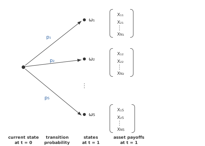
Arrow-Debreu Securities¶
Definition¶
Definition: Arrow-Debreu Security
An Arrow-Debreu security (also called a pure state security or primitive security) for state \(s\) is a financial contract that pays exactly 1 unit of currency if state \(\omega_s\) occurs and 0 in all other states.
Formally, the Arrow-Debreu security for state \(s\) has the payoff vector:
If we have \(S\) states, there are \(S\) possible Arrow-Debreu securities \(\mathbf{e}_1, \mathbf{e}_2, \ldots, \mathbf{e}_S\), which together form the identity matrix \(\mathbf{I}_S\).
Intuition¶
Arrow-Debreu securities isolate and "price" individual states of the world. They decompose uncertainty into its most elementary components. Any asset with an arbitrary payoff profile can be viewed as a portfolio of Arrow-Debreu securities:
This makes Arrow-Debreu securities the "building blocks" of all financial claims.
Example: Two-State Economy
Suppose the economy has two states: Boom (\(\omega_1\)) and Recession (\(\omega_2\)).
- The Arrow-Debreu security for Boom pays \((1, 0)\): you receive $1 if the economy booms, $0 otherwise.
- The Arrow-Debreu security for Recession pays \((0, 1)\): you receive $1 if recession occurs, $0 otherwise.
A stock that pays $120 in Boom and $80 in Recession is equivalent to holding 120 units of the Boom Arrow-Debreu security and 80 units of the Recession Arrow-Debreu security.
State Prices¶
Definition¶
Definition: State Price
The state price \(\phi_s\) is the price at \(t = 0\) of the Arrow-Debreu security for state \(s\). That is, \(\phi_s\) is the cost today of receiving $1 if and only if state \(\omega_s\) occurs at \(t = 1\).
The vector of state prices is:
Pricing Any Asset with State Prices¶
If state prices exist, the price of any asset \(j\) with payoffs \((X_{j1}, X_{j2}, \ldots, X_{jS})\) is simply:
This is the fundamental pricing equation. It says that an asset's price equals the sum of its payoffs in each state, weighted by the state prices.
In matrix form for all \(N\) assets:
where \(\mathbf{P} = (P_1, P_2, \ldots, P_N)^\top\) is the vector of asset prices.
Two Properties of \(\boldsymbol{\phi}\)¶
Under no-arbitrage, the FTAP gives positivity: \(\phi_s > 0\) for every \(s\). Economically, every state is "valuable" — investors are willing to pay a positive price for insurance against any possible state.
The risk-free bond pays \(1 + r_f\) in every state at price \(1\). Applying \(P = \boldsymbol{\phi}^\top \mathbf{X}_j\) to this row gives the bond identity:
so the state prices sum to the discount factor \(\beta\). In particular \(\sum_s \phi_s < 1\) when \(r_f > 0\). This identity is the bridge from \(\boldsymbol{\phi}\) to the risk-neutral measure below.
State Prices and Risk-Neutral Pricing¶
Constructing the Risk-Neutral Measure¶
State prices naturally give rise to risk-neutral probabilities. Define:
Since \(\phi_s > 0\) for all \(s\) and \(\sum_s q_s = 1\), the \(q_s\) form a valid probability measure \(\mathbb{Q}\), called the risk-neutral measure (or equivalent martingale measure).
Risk-Neutral Pricing Formula¶
Under \(\mathbb{Q}\), the fundamental pricing equation becomes:
Interpretation
Under the risk-neutral measure, every asset earns the risk-free rate in expectation. The asset price equals the discounted expected payoff under \(\mathbb{Q}\). This is not because investors are risk-neutral — rather, risk aversion is already embedded in the distortion from \(p_s\) to \(q_s\).
Comparing Physical and Risk-Neutral Probabilities¶
| State | Physical Prob. \(p_s\) | State Price \(\phi_s\) | Risk-Neutral Prob. \(q_s\) |
|---|---|---|---|
| Boom | High | Low (relative to \(p_s\)) | Low |
| Recession | Low | High (relative to \(p_s\)) | High |
Risk-neutral probabilities overweight bad states (where marginal utility is high) and underweight good states relative to physical probabilities. This reflects the market's aggregate risk aversion.
Stochastic Discount Factor (Pricing Kernel)¶
The stochastic discount factor (SDF), also called the pricing kernel, connects state prices to physical probabilities:
The SDF allows us to write the pricing equation using physical probabilities:
Interpretation of the SDF
- \(m_s\) reflects the marginal rate of substitution between consumption today and consumption in state \(s\).
- In equilibrium models (e.g., CCAPM), \(m_s = \beta \frac{u'(C_1(\omega_s))}{u'(C_0)}\), where \(\beta\) is the time discount factor and \(u\) is the utility function.
- The SDF is high in "bad" states (low consumption) and low in "good" states (high consumption).
Relationships Summary¶
The three representations — state prices, risk-neutral probabilities, and the SDF — are equivalent ways to enforce no-arbitrage:
| Representation | Pricing Formula | Key Object |
|---|---|---|
| State Prices | \(P = \sum_s \phi_s X_s\) | \(\phi_s\) |
| Risk-Neutral | \(P = \frac{1}{1+r_f}\mathbb{E}^{\mathbb{Q}}[X]\) | \(q_s\) |
| SDF / Pricing Kernel | \(P = \mathbb{E}^{\mathbb{P}}[m \cdot X]\) | \(m_s\) |
Completeness and Uniqueness of State Prices¶
Recall (see § Portfolios and payoffs): the market is complete iff \(\operatorname{rank}(\mathbf{X}) = S\), i.e. every payoff vector \(\mathbf{c} \in \mathbb{R}^S\) is replicable.
Theorem: Completeness \(\iff\) Unique State Prices
Under no-arbitrage, the state price vector \(\boldsymbol{\phi} \gg \mathbf{0}\) with \(\mathbf{P} = \mathbf{X}\boldsymbol{\phi}\) is unique iff the market is complete. In the incomplete case, infinitely many positive \(\boldsymbol{\phi}\) (and hence risk-neutral measures \(\mathbb{Q}\) and SDFs \(m\)) are consistent with the observed prices, and non-attainable claims have a range of no-arbitrage prices rather than a single one.
The proof and the pricing-interval consequences in the incomplete case are the subject of the Second FTAP: see § Complete Markets and Uniqueness.
Extracting State Prices from Market Data¶
From Observed Prices¶
Given \(N\) assets with price vector \(\mathbf{P}\) and payoff matrix \(\mathbf{X}\), state prices solve:
- If \(N = S\) and \(\mathbf{X}\) has full rank: \(\boldsymbol{\phi} = \mathbf{X}^{-1} \mathbf{P}\) (unique solution).
- If \(N > S\): overdetermined system; use least squares or check consistency.
- If \(N < S\): underdetermined; infinitely many solutions (incomplete market).
Numerical Example¶
Extracting State Prices: Two-State Example
Consider two states (Boom, Recession) and two assets:
- Risk-free bond: Price = $0.95, pays $1 in both states.
- Stock: Price = $50, pays $70 in Boom, $40 in Recession.
The payoff matrix and price vector are:
Solving \(\mathbf{X} \boldsymbol{\phi} = \mathbf{P}\):
From the first equation: \(\phi_2 = 0.95 - \phi_1\). Substituting:
Results:
| Boom (\(\omega_1\)) | Recession (\(\omega_2\)) | |
|---|---|---|
| State Price \(\phi_s\) | 0.40 | 0.55 |
| Risk-Neutral Prob. \(q_s = \phi_s / 0.95\) | 0.4211 | 0.5789 |
Note that \(\phi_2 > \phi_1\): the market prices recession insurance more highly than boom insurance, reflecting aggregate risk aversion. The risk-neutral probability of recession (0.5789) exceeds its physical probability (which might be, say, 0.3), distorting probabilities toward the "bad" state.
From Option Prices: The Breeden-Litzenberger Result¶
In continuous-state settings, state prices can be extracted from European option prices. If \(C(K)\) denotes the price of a European call option with strike \(K\) on an asset with terminal price \(S_T\), and the state price density is \(\phi(s)\), then:
Differentiating twice with respect to \(K\):
This is the Breeden-Litzenberger formula. It shows that the curvature of the call price function with respect to the strike price reveals the state price density (and hence the risk-neutral density).
Practical Implication
Butterfly spreads (long calls at \(K - \Delta K\) and \(K + \Delta K\), short two calls at \(K\)) approximate \(\frac{\partial^2 C}{\partial K^2}\) and thus provide discrete estimates of state prices. This is the basis for extracting implied risk-neutral distributions from option markets.
Connections to Other Topics¶
Broader Context
State prices and Arrow-Debreu securities connect to many central topics in financial mathematics:
- Risk-Neutral Valuation: State prices provide the discrete foundation for the risk-neutral pricing approach used in continuous-time models (Black-Scholes, etc.).
- Fundamental Theorems of Asset Pricing: The existence and uniqueness of state prices correspond to the first and second fundamental theorems.
- Derivative Pricing: Options and other derivatives are priced as portfolios of Arrow-Debreu securities.
- Term Structure Models: State prices across maturities determine the yield curve and the prices of zero-coupon bonds.
- Portfolio Theory: Complete markets allow perfect hedging; incomplete markets require optimization under constraints.
- Consumption-Based Models: The SDF interpretation links asset pricing to macroeconomic fundamentals via the Euler equation.
Summary¶
| Concept | Definition | Key Formula |
|---|---|---|
| Arrow-Debreu Security | Pays $1 in one state, $0 otherwise | Payoff \(= \mathbf{e}_s\) |
| State Price \(\phi_s\) | Price of the Arrow-Debreu security for state \(s\) | \(P_j = \sum_s \phi_s X_{js}\) |
| Risk-Neutral Probability \(q_s\) | \(\phi_s\) rescaled to sum to 1 | \(q_s = \phi_s(1+r_f)\) |
| Stochastic Discount Factor \(m_s\) | State price per unit probability | \(m_s = \phi_s / p_s\) |
| Complete Market | Every payoff is replicable | \(\text{rank}(\mathbf{X}) = S\) |
| Breeden-Litzenberger | State prices from option prices | \(\phi(K) = e^{rT} \partial^2 C / \partial K^2\) |
Exercises¶
Exercise 1. Consider a two-state economy with states \(\Omega = \{\omega_1, \omega_2\}\). A risk-free bond has price \(P_{\text{rf}} = 0.90\) and pays $1 in both states. A stock has price \(P_2 = 60\) and pays $80 in state \(\omega_1\) and $50 in state \(\omega_2\). Compute the state prices \(\phi_1\) and \(\phi_2\), the risk-neutral probabilities \(q_1\) and \(q_2\), and the stochastic discount factor values \(m_1\) and \(m_2\) assuming physical probabilities \(p_1 = 0.5\) and \(p_2 = 0.5\).
Solution to Exercise 1
State prices: Solve \(\mathbf{X}\,\boldsymbol{\phi} = \mathbf{P}\):
From equation (1): \(\phi_2 = 0.90 - \phi_1\). Substituting into equation (2):
Risk-neutral probabilities: The risk-free rate satisfies \(1/(1 + r_f) = \sum_s \phi_s = 0.90\), so \(r_f = 1/0.90 - 1 = 10/9 - 1 = 1/9 \approx 0.1111\) (about \(11.11\%\)). Then:
Stochastic discount factor: With \(p_1 = p_2 = 0.5\):
Verification: \(P_2 = \mathbb{E}^{\mathbb{P}}[m \cdot X_2] = 0.5(1.00)(80) + 0.5(0.80)(50) = 40 + 20 = 60\). Correct.
Note that \(m_2 < m_1\): the SDF is lower in the recession state, which is unusual. Typically the SDF is higher in bad states (reflecting higher marginal utility). Here the "recession" state has a lower SDF, which could occur if the economy has unusual risk preferences or if state \(\omega_2\) is not truly the "bad" state in terms of aggregate consumption.
Exercise 2. Prove that if no-arbitrage holds and a risk-free bond exists paying $1 in every state, then the sum of the state prices satisfies
where \(r_f\) is the risk-free rate. What does this imply about the relationship between state prices and risk-neutral probabilities?
Solution to Exercise 2
Suppose a risk-free bond exists with payoff \(X_{\text{rf},s} = 1\) for all \(s = 1, \ldots, S\) and price \(P_{\text{rf}}\). The fundamental pricing equation gives:
The risk-free bond has gross return \((1 + r_f)\), meaning:
(investing \(P_{\text{rf}}\) today yields $1 in every state, so the gross return is \(1/P_{\text{rf}} = 1 + r_f\)). Combining:
Implication for risk-neutral probabilities: Define \(q_s = \phi_s (1 + r_f)\) for each \(s\). Then:
Since \(\phi_s > 0\) (no-arbitrage), we have \(q_s > 0\) for all \(s\). Therefore the \(q_s\) form a valid probability measure. This is the risk-neutral measure \(\mathbb{Q}\), and the state prices are precisely the discounted risk-neutral probabilities: \(\phi_s = q_s / (1 + r_f)\).
Exercise 3. In a three-state economy with \(\Omega = \{\omega_1, \omega_2, \omega_3\}\), the payoff matrix and price vector are
Solve \(\mathbf{X}\,\boldsymbol{\phi} = \mathbf{P}\) for the state price vector \(\boldsymbol{\phi}\). Verify that all components are strictly positive and compute the implied risk-free rate.
Solution to Exercise 3
We solve the system \(\mathbf{X}\,\boldsymbol{\phi} = \mathbf{P}\):
Note that equation (2) equals \(10 \times\) equation (1) plus \(50\phi_1 + 40\phi_2 + 30\phi_3\)... Let us solve directly.
Subtract \(40 \times\) equation (1) from equation (2):
So \(2\phi_1 + \phi_2 = 0.96\).
From equation (3): \(10\phi_1 + 5\phi_2 = 4.80\), so \(2\phi_1 + \phi_2 = 0.96\) ... (ii).
Equations (i) and (ii) are identical: \(2\phi_1 + \phi_2 = 0.96\). This means we have one free parameter. Let \(\phi_1 = t\). Then \(\phi_2 = 0.96 - 2t\) and from equation (1): \(\phi_3 = 0.96 - t - (0.96 - 2t) = t\).
So \(\boldsymbol{\phi} = (t,\; 0.96 - 2t,\; t)^\top\).
For strict positivity: \(t > 0\), \(0.96 - 2t > 0 \implies t < 0.48\), and \(t > 0\). So \(t \in (0, 0.48)\).
For example, choosing \(t = 0.16\): \(\boldsymbol{\phi} = (0.16,\; 0.64,\; 0.16)^\top\).
Verification: \(\phi_1 + \phi_2 + \phi_3 = 0.16 + 0.64 + 0.16 = 0.96\). Check equation (2): \(60(0.16) + 50(0.64) + 40(0.16) = 9.6 + 32 + 6.4 = 48\). Check equation (3): \(10(0.16) + 5(0.64) = 1.6 + 3.2 = 4.8\). All correct.
All components are strictly positive for any \(t \in (0, 0.48)\), confirming the market is arbitrage-free.
Implied risk-free rate:
Note that the state prices are not unique (the market has 3 states but the system has only 2 independent equations from 3 assets), confirming the market is incomplete.
Exercise 4. Show that the stochastic discount factor \(m_s = \phi_s / p_s\) satisfies
when a risk-free bond exists. Interpret this result in terms of the relationship between the SDF and the time value of money.
Solution to Exercise 4
The SDF is \(m_s = \phi_s / p_s\). Taking the expectation under the physical measure \(\mathbb{P}\):
When a risk-free bond exists (as shown in Exercise 2):
Therefore:
Interpretation: The expected value of the SDF under the physical measure equals the discount factor. This means the SDF "on average" discounts future payoffs at the risk-free rate. Applying the SDF pricing formula to the risk-free bond with constant payoff $1:
This confirms that the time value of money (as captured by \(r_f\)) is embedded in the average level of the SDF. The SDF fluctuates around its mean \(1/(1 + r_f)\), being higher in bad states and lower in good states. This state-dependence is what distinguishes risky asset pricing from riskless discounting.
Exercise 5. A market has two states and two traded assets (a bond and a stock). The state prices are \(\phi_1 = 0.35\) and \(\phi_2 = 0.60\). A new derivative is introduced with payoff \(\Phi(\omega_1) = 10\) and \(\Phi(\omega_2) = 3\). Using the fundamental pricing equation, compute the no-arbitrage price of this derivative. Then verify your answer using the risk-neutral pricing formula \(P = \frac{1}{1+r_f}\mathbb{E}^{\mathbb{Q}}[\Phi]\).
Solution to Exercise 5
Using the fundamental pricing equation:
Verification via risk-neutral pricing: First, find the risk-free rate:
The risk-neutral probabilities are:
The risk-neutral expected payoff is:
The discounted expected payoff is:
Both methods give the same no-arbitrage price of $5.30.
Exercise 6. Explain why the Breeden-Litzenberger formula \(\phi(K) = e^{r_f T} \frac{\partial^2 C}{\partial K^2}\) implies that the call price \(C(K)\) must be a convex function of the strike price \(K\) in an arbitrage-free market. What would a violation of convexity imply about state prices?
Solution to Exercise 6
The Breeden-Litzenberger formula states:
In an arbitrage-free market, state prices must be strictly positive: \(\phi(K) > 0\) for all \(K\) in the support of the asset's terminal distribution. Since \(e^{r_f T} > 0\), positivity of \(\phi(K)\) requires:
This is precisely the condition that \(C(K)\) is a convex function of \(K\). (A twice-differentiable function is convex if and only if its second derivative is non-negative everywhere.)
What a violation of convexity would imply: If \(C(K)\) were not convex at some strike \(K_0\), then \(\frac{\partial^2 C}{\partial K^2}\big|_{K_0} < 0\), which would give \(\phi(K_0) < 0\). A negative state price means the market assigns a negative value to receiving $1 in a particular state of the world. This is economically absurd and constitutes an arbitrage opportunity.
Concretely, a violation of convexity can be exploited via a butterfly spread: buy calls at strikes \(K_0 - \Delta K\) and \(K_0 + \Delta K\), and sell two calls at strike \(K_0\). If \(C(K)\) is locally concave at \(K_0\), this butterfly spread has a negative cost (you receive a net premium) but a non-negative payoff in every state. This is a Type 2 arbitrage. Therefore, in an arbitrage-free market, call prices must be convex in the strike price.