Simulations
This page consolidates all computational experiments for the simple random walk. The simulations verify the theoretical properties derived in earlier sections. Each block is self-contained and can be run independently.
Simulation 1: Single Path
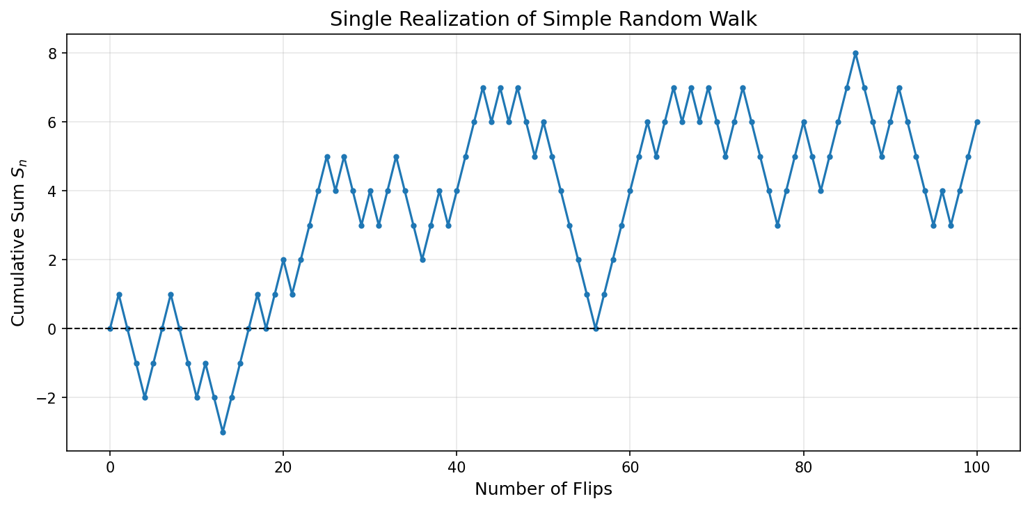
A single realization of a simple symmetric random walk over 100 steps.
```python import matplotlib.pyplot as plt import numpy as np
np.random.seed(42)
num_flips = 100 flips = np.random.choice([1, -1], size=num_flips) heads_count = np.sum(flips == 1) tails_count = np.sum(flips == -1) print(f"Heads: {heads_count}, Tails: {tails_count}")
cumsum_flips = np.cumsum(np.insert(flips, 0, 0))
fig, ax = plt.subplots(figsize=(10, 5)) ax.plot(cumsum_flips, marker='o', linestyle='-', markersize=3) ax.set_xlabel("Number of Flips", fontsize=12) ax.set_ylabel("Cumulative Sum \(S_n\)", fontsize=12) ax.set_title("Single Realization of Simple Random Walk", fontsize=14) ax.axhline(0, color='black', linestyle='--', linewidth=1) ax.grid(alpha=0.3) plt.tight_layout() plt.show()
print(f"Final position S_100 = {cumsum_flips[-1]}") ```
Output:
Heads: 53, Tails: 47
Final position S_100 = 6
What to observe:
- The path oscillates around zero, consistent with \(\mathbb{E}[S_n] = 0\).
- Final position \(S_{100} = 6\) is of order \(\sqrt{100} = 10\), consistent with \(\text{SD}(S_n) = \sqrt{n}\).
- Every step produces a "kink" — no tangent exists anywhere, foreshadowing the nowhere-differentiability of Brownian motion.
Simulation 2: Scaled Walk Converging to Brownian Motion
Donsker's theorem predicts \(W^{(n)} \Rightarrow W\) in \(C[0,1]\) as \(n \to \infty\). As \(n\) increases, the piecewise-linear paths become finer and approach the visual character of Brownian motion.
```python import matplotlib.pyplot as plt import numpy as np
Hierarchical construction: generate one base path at n_base=1000 steps, then
display the same path at three resolutions by subsampling every 'step' positions.
Normalisation: dividing by sqrt(n_base) gives variance ≈ t on [0,1] at all resolutions,
since Var(S_base[kstep]) = kstep, and kstep/n_base = t at time t = kstep/n_base.
np.random.seed(42) T = 1.0 n_base = 1000 # finest discretization num_paths = 5
fig, axes = plt.subplots(1, 3, figsize=(15, 4)) subsample_levels = [10, 100, 1000]
for _ in range(num_paths): xi_base = np.random.choice([1, -1], size=n_base) S_base = np.cumsum(np.insert(xi_base, 0, 0)) # length n_base + 1
for idx, n in enumerate(subsample_levels):
    step = n_base // n        # e.g. step=100 for n=10, step=1 for n=1000
    t = np.linspace(0, T, n + 1)
    S_sub = S_base[::step]   # subsample: n+1 positions
    # Divide by sqrt(n_base) so that Var(S_sub[k] / sqrt(n_base)) = k*step/n_base = t_k
    axes[idx].plot(t, S_sub / np.sqrt(n_base), alpha=0.7, linewidth=1.5)
for idx, n in enumerate(subsample_levels): axes[idx].set_title(f'\(n = {n}\) steps', fontsize=11) axes[idx].set_xlabel('Time \(t\)', fontsize=10) axes[idx].set_ylabel(r'\(S_{\lfloor n_{\rm base}\,t\rfloor}/\sqrt{n_{\rm base}}\)', fontsize=10) axes[idx].axhline(0, color='black', linestyle='--', linewidth=0.8, alpha=0.5) axes[idx].grid(alpha=0.3) axes[idx].set_ylim(-2.5, 2.5)
plt.suptitle("The Same Path at Three Resolutions (Donsker's Theorem)", fontsize=14, fontweight='bold') plt.tight_layout() plt.show() ```
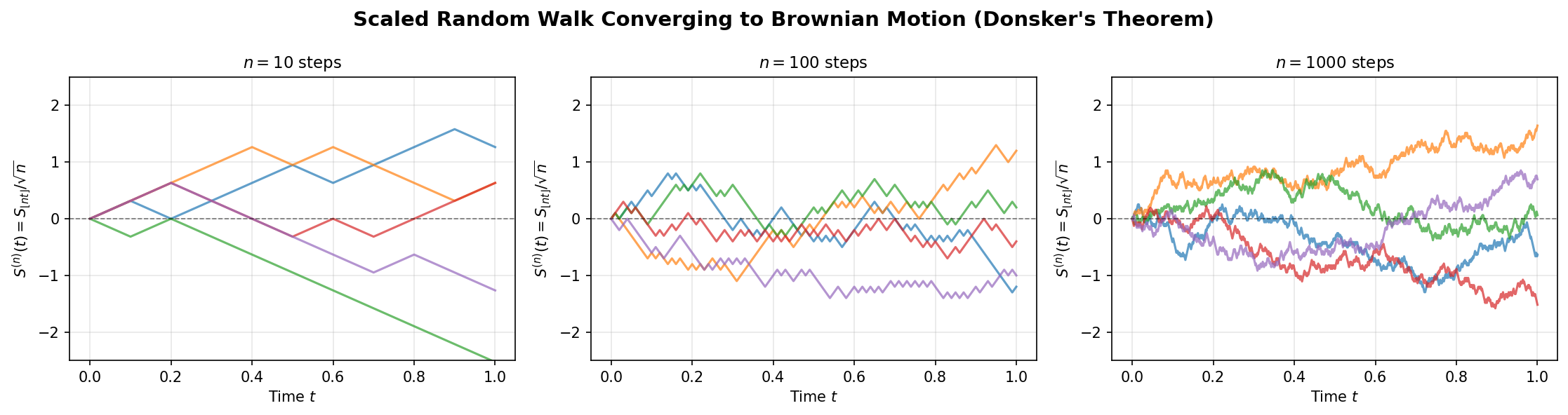
What to observe: The same underlying base path (1000 steps) is shown subsampled at three resolutions. All three panels display \(S_{\lfloor n_\text{base}\,t \rfloor}/\sqrt{n_\text{base}}\), so the vertical scale is identical across panels — each has variance \(\approx t\). The visual difference is in horizontal resolution: at \(n = 10\) the path has only 10 plotted points and the coarse steps are clearly visible; at \(n = 1000\) all base steps are plotted and the path appears visually continuous. This illustrates the key message of Donsker's theorem: as we observe the walk at finer time-scales, the path character approaches that of Brownian motion.
| \(n\) | Plotted points | Interval between points | Visual character |
|---|---|---|---|
| 10 | 11 | \(T/10 = 0.1\) | Coarse, stepped |
| 100 | 101 | \(T/100 = 0.01\) | Smoother |
| 1000 | 1001 | \(T/1000 = 0.001\) | Visually continuous |
Simulation 3: Quadratic Variation
Proposition 1.1.5 states \([S]_n = n\) almost surely — deterministically, not as a statistical average. This simulation makes that striking fact visual.
```python import matplotlib.pyplot as plt import numpy as np
np.random.seed(42)
num_steps = 1000 num_paths = 20
QV_paths = np.zeros((num_paths, num_steps)) for k in range(num_paths): xi = np.random.choice([1, -1], size=num_steps) S = np.cumsum(np.insert(xi, 0, 0)) QV_paths[k, :] = np.cumsum(np.diff(S)**2)
n_range = range(1, num_steps + 1)
fig, ax = plt.subplots(figsize=(9, 5)) for i in range(num_paths): ax.plot(n_range, QV_paths[i, :], alpha=0.4, linewidth=1) ax.plot(n_range, list(n_range), 'r--', linewidth=2.5, label='\([S]_n = n\) (theoretical)', zorder=5) ax.set_xlabel('Time step \(n\)', fontsize=12) ax.set_ylabel('Quadratic Variation \([S]_n\)', fontsize=12) ax.set_title('Quadratic Variation of the Random Walk', fontsize=13) ax.legend(fontsize=11) ax.grid(alpha=0.3) plt.tight_layout() plt.show()
print(f"All paths equal n exactly: {np.allclose(QV_paths[:, -1], num_steps)}") ```
Output:
All paths equal n exactly: True
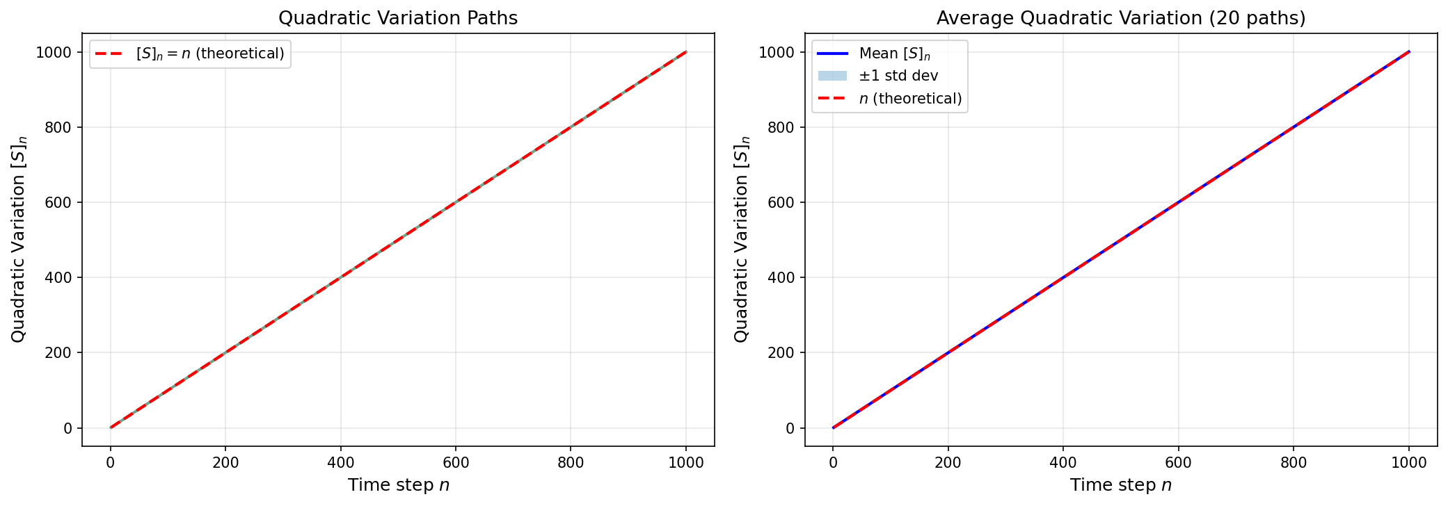
What to observe: Every colored path lies exactly on the red dashed line \([S]_n = n\). There is no spread — the quadratic variation has zero randomness. The contrast with \(S_n\) itself (which has spread \(\sim\sqrt{n}\)) illustrates why \([S]_n = n\) is a structural property: it holds because \(\xi_i^2 = 1\) always, regardless of the sign of \(\xi_i\).
Exercises
Exercise 1. Modify Simulation 1 to generate an asymmetric random walk with \(p = 0.55\). Run 100 steps and plot the result. Compute the sample mean and compare it to the theoretical value \(\mathbb{E}[S_{100}] = 100(2 \cdot 0.55 - 1) = 10\). Does the upward drift become visually apparent in a single path?
Solution to Exercise 1
Modify the random step generation to use unequal probabilities:
python
flips = np.random.choice([1, -1], size=100, p=[0.55, 0.45])
The theoretical mean is \(\mathbb{E}[S_{100}] = 100(2 \cdot 0.55 - 1) = 10\) and standard deviation is \(\sqrt{4 \cdot 100 \cdot 0.55 \cdot 0.45} = \sqrt{99} \approx 9.95\).
In a single path, the drift may or may not be visually apparent: the expected position (10) is only about 1 standard deviation above 0, so a single realization could plausibly end negative. With multiple paths the upward trend becomes clear, but for a single path the noise-to-signal ratio at \(n = 100\) is still significant.
Exercise 2. Write a simulation to verify that the quadratic variation of the scaled random walk \(S^{(n)}(t) = S_{\lfloor nt \rfloor}/\sqrt{n}\) converges to \(t\) as \(n\) increases. Use \(t = 1\) and \(n = 10, 100, 1000, 10000\). For each \(n\), compute \([S^{(n)}]_1 = \lfloor n \rfloor / n\) and verify it equals 1 (or very close to 1 for non-integer \(nt\)).
Solution to Exercise 2
For \(t = 1\) and integer \(n\), the quadratic variation of the scaled walk is:
exactly, for all \(n\). This holds because \(nt = n\) is an integer when \(t = 1\), so \(\lfloor nt \rfloor = n\) exactly. The simulation code:
python
for n in [10, 100, 1000, 10000]:
    xi = np.random.choice([1, -1], size=n)
    QV = np.sum((xi / np.sqrt(n))**2)
    print(f"n = {n}: [S^(n)]_1 = {QV:.6f}")
Every output will be exactly 1.000000, because each \((xi_i/\sqrt{n})^2 = 1/n\), and there are \(n\) terms, giving \(n \cdot (1/n) = 1\).
Exercise 3. Write a simulation to estimate the distribution of the maximum of a symmetric random walk over \(n = 1000\) steps: \(M_n = \max_{0 \leq k \leq n} S_k\). Generate 10,000 paths and plot the histogram of \(M_n / \sqrt{n}\). Compare your histogram to the theoretical distribution \(\mathbb{P}(\max_{0 \leq t \leq 1} W_t \leq x) = 2\Phi(x) - 1\) for \(x \geq 0\) (which follows from the reflection principle of Brownian motion).
Solution to Exercise 3
The simulation generates 10,000 paths of length \(n = 1000\) and records \(M_n = \max_{0 \leq k \leq n} S_k\) for each. The histogram of \(M_n/\sqrt{n}\) should approximate the theoretical CDF:
The corresponding density (for \(x > 0\)) is:
where \(\phi\) is the standard normal density. This is a half-normal distribution (the distribution of \(|Z|\) where \(Z \sim \mathcal{N}(0,1)\)). The histogram should show a distribution concentrated on \([0, \infty)\) with mode at 0 and right-skewed tail, matching \(2\phi(x)\).
Exercise 4. Use Simulation 2 (scaled walk convergence) as a starting point. Generate 1000 paths of the scaled walk \(W^{(n)}\) for \(n = 500\) and compute the sample distribution of \(W^{(n)}(0.5)\). Plot the histogram and overlay the theoretical density \(\mathcal{N}(0, 0.5)\). This provides a visual verification of the CLT at the intermediate time \(t = 0.5\).
Solution to Exercise 4
With \(n = 500\) and \(t = 0.5\): \(S^{(n)}(0.5) = S_{\lfloor 250 \rfloor}/\sqrt{500} = S_{250}/\sqrt{500}\). By the CLT, \(S_{250}/\sqrt{250} \approx \mathcal{N}(0,1)\), so \(S_{250}/\sqrt{500} = (S_{250}/\sqrt{250}) \cdot \sqrt{250/500} \approx \mathcal{N}(0,1) \cdot (1/\sqrt{2})\), which gives \(\mathcal{N}(0, 1/2) = \mathcal{N}(0, 0.5)\).
The histogram of 1000 samples of \(W^{(500)}(0.5)\) should match the density:
The distribution is centred at 0 with standard deviation \(\sqrt{0.5} \approx 0.707\). The overlay of the theoretical \(\mathcal{N}(0, 0.5)\) density should closely match the histogram, confirming the CLT at \(t = 0.5\).