Girsanov's Theorem¶
Girsanov's theorem is one of the most powerful tools in mathematical finance. It describes how a change of probability measure modifies the drift of a stochastic process while preserving its Brownian structure. This is essential for pricing derivatives via risk-neutral measures.
Toy mechanism: one likelihood ratio fixes everything
Recall (see § Intuitive Introduction) the discrete picture: changing \(\mathbb{P}(H) = p\) to \(\mathbb{Q}(H) = q\) amounts to multiplying by the likelihood ratio \(L = \mathbb{Q}/\mathbb{P}\), then \(\mathbb{E}^{\mathbb{Q}}[X] = \mathbb{E}^{\mathbb{P}}[LX]\). Girsanov's theorem promotes this single line of arithmetic to a Brownian filtration: the density \(Z_T\) defined below plays the role of \(L\), and its construction is reverse-engineered so that the shifted process \(\widetilde W_t = W_t + \int_0^t\theta_s\,ds\) becomes a \(\mathbb{Q}\)-Brownian motion. Three numbered boxes follow — exponential martingale, measure change, statement — and they are the only nontrivial content of the theorem.
Standing assumptions
All processes in this section are defined on a filtered probability space \((\Omega, \mathcal{F}, \{\mathcal{F}_t\}, \mathbb{P})\) satisfying the usual conditions. All measure changes are between equivalent probability measures (\(\mathbb{Q} \sim \mathbb{P}\)), meaning they share the same null sets: events impossible under \(\mathbb{P}\) remain impossible under \(\mathbb{Q}\), and vice versa. Throughout, we distinguish local martingales from true martingales; the latter requires integrability verification (e.g., Novikov's condition).
Notation convention
Throughout this section, \(\theta_t\) denotes the Girsanov kernel (drift adjustment process). In financial applications, \(\theta_t = (\mu_t - r_t)/\sigma_t\) is the market price of risk. Some references use \(\lambda_t\) for the same quantity; in the interest rate literature \(\lambda\) is the conventional symbol for the market price of interest rate risk.
Setting and Assumptions¶
Let \((\Omega, \mathcal{F}, \{\mathcal{F}_t\}, \mathbb{P})\) be a filtered probability space supporting a standard Brownian motion \(W_t\).
Let \(\theta_t\) be an adapted process (the Girsanov kernel) satisfying the Novikov condition:
This condition ensures that the exponential martingale does not explode and is a true martingale (not just a local martingale).
The Exponential Martingale¶
Define the Radon–Nikodym derivative (also called the exponential martingale):
Key properties:
- Strictly positive: \(Z_t > 0\) almost surely for all \(t\)
- Martingale: Under the original measure \(\mathbb{P}\), \(Z_t\) is a true martingale
- Unit expectation: \(\mathbb{E}^{\mathbb{P}}[Z_t] = 1\) for all \(t\)
The Measure Change¶
Define a new probability measure \(\mathbb{Q}\) on \(\mathcal{F}_T\) via:
For any \(\mathcal{F}_T\)-measurable random variable \(X\) with \(\mathbb{E}^{\mathbb{P}}[|X| \cdot Z_T] < \infty\), the relationship between expectations under the two measures is:
If in addition \(X\) is \(\mathcal{F}_t\)-measurable for some \(t \leq T\), then since \(Z_s\) is a \(\mathbb{P}\)-martingale we can replace \(Z_T\) by \(Z_t\):
In particular, taking \(X = \mathbf{1}_A\) for \(A \in \mathcal{F}_t\):
Statement of Girsanov's Theorem¶
Theorem (Girsanov, 1960): Under the new measure \(\mathbb{Q}\), the process
is a standard Brownian motion.
Interpretation: How the Drift Term Changes¶
| Perspective | Under \(\mathbb{P}\) (Original Measure) | Under \(\mathbb{Q}\) (New Measure) |
|---|---|---|
| Brownian motion | \(W_t\) is standard | \(\widetilde{W}_t\) is standard |
| Transformed BM | \(\widetilde{W}_t = W_t + \int \theta\,ds\) has drift | Driftless |
| What changed | Original measure | Probability measure (and hence the law of the process) |
| Information structure | Same filtration | Same filtration |
| Volatility | Unchanged | Unchanged |
See Intuitive Introduction for conceptual interpretation, Proof Sketch for derivation, and Drift Adjustment for financial application.
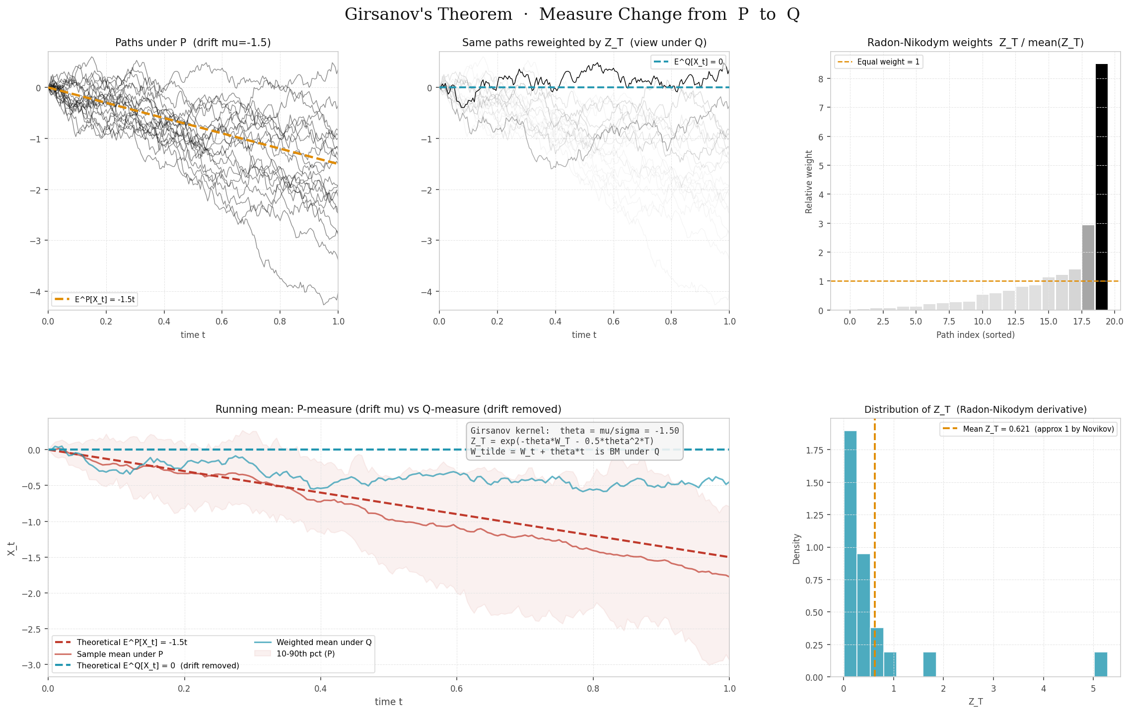
Application¶
For drift removal in SDEs, the GBM worked example, and the risk-neutral pricing formula, see Drift Adjustment and Financial Meaning.
Python: Simulating the Measure Change¶
The following script reproduces Figure 1. It simulates 200 drifted Brownian motion paths under \(\mathbb{P}\), computes the Radon–Nikodym weights \(Z_T\), and visualizes the measure change in six panels. In the path panels, opacity encodes the weight: high-\(Z_T\) paths appear dark and prominent, while low-\(Z_T\) paths fade out, making the measure change immediately visible.
Dependencies: numpy, matplotlib
```python """ Girsanov's Theorem – Visualization ==================================== Simulates drifted BM paths under P, computes Radon-Nikodym weights Z_T, and displays the measure change P → Q in six panels (reproduces Figure 1). """
import numpy as np import matplotlib.pyplot as plt import matplotlib.gridspec as gridspec
── Parameters ────────────────────────────────────────────────────────────────¶
RNG = np.random.default_rng(42) N_PATHS = 200 # number of simulated paths N_STEPS = 200 # discretisation steps T = 1.0 # terminal time MU = -1.5 # drift under P (negative, as in the Wikipedia figure) SIGMA = 1.0 # diffusion coefficient dt = T / N_STEPS t_grid = np.linspace(0, T, N_STEPS + 1)
── Simulate paths under P: X_t = μt + σW_t ──────────────────────────────────¶
dW = RNG.standard_normal((N_PATHS, N_STEPS)) * np.sqrt(dt) W = np.hstack([np.zeros((N_PATHS, 1)), np.cumsum(dW, axis=1)]) X_P = MU * t_grid + SIGMA * W
── Girsanov kernel and Radon-Nikodym weights ─────────────────────────────────¶
Choose θ = μ/σ so that the drift is completely removed under Q.¶
theta = MU / SIGMA # = -1.5 here
Z_T = exp(−θ W_T − ½ θ² T) [constant θ → stochastic integral = θ·W_T]¶
Z_T = np.exp(-theta * W[:, -1] - 0.5 * theta**2 * T) Z_norm = Z_T / Z_T.mean() # relative weights (mean ≈ 1)
── Weighted mean under Q ─────────────────────────────────────────────────────¶
mean_P = X_P.mean(axis=0) mean_Q = (X_P * Z_T[:, None]).sum(axis=0) / Z_T.sum()
── Figure layout ─────────────────────────────────────────────────────────────¶
AMBER_C = "#e08b00" BLUE_C = "#2196b0" RED_C = "#c0392b" GRID_C = "#e5e5e5"
fig = plt.figure(figsize=(16, 10), facecolor="white") fig.suptitle( "Girsanov's Theorem · Measure Change from P to Q", fontsize=16, color="#111", fontfamily="serif", y=0.98 ) gs = gridspec.GridSpec(2, 3, figure=fig, hspace=0.42, wspace=0.35, left=0.06, right=0.96, top=0.92, bottom=0.08)
ax_P = fig.add_subplot(gs[0, 0]) # paths under P ax_Q = fig.add_subplot(gs[0, 1]) # reweighted paths (view under Q) ax_wt = fig.add_subplot(gs[0, 2]) # weight bar chart ax_mean = fig.add_subplot(gs[1, :2]) # running mean P vs Q ax_zd = fig.add_subplot(gs[1, 2]) # Z_T histogram
for ax in [ax_P, ax_Q, ax_wt, ax_mean, ax_zd]: ax.set_facecolor("white") for spine in ax.spines.values(): spine.set_color("#ccc") ax.tick_params(colors="#444", labelsize=8) ax.xaxis.label.set_color("#444") ax.yaxis.label.set_color("#444") ax.title.set_color("#111") ax.grid(color=GRID_C, linewidth=0.5, linestyle="--")
── Panel 1: paths under P — equal alpha, black lines ────────────────────────¶
for i in range(N_PATHS): ax_P.plot(t_grid, X_P[i], color="black", lw=0.5, alpha=0.25)
ax_P.plot(t_grid, MU * t_grid, color=AMBER_C, lw=2.2, ls="--", label="E^P[X_t] = {}t".format(MU), zorder=5) ax_P.set_xlim(0, T) ax_P.set_ylim(X_P.min() - 0.1, X_P.max() + 0.1) ax_P.set_title("Paths under P (drift mu={})".format(MU), fontsize=10, pad=6) ax_P.set_xlabel("time t", fontsize=8) ax_P.legend(fontsize=7, loc="lower left", framealpha=0.6)
── Panel 2: same paths reweighted by Z_T — alpha ∝ Z_norm ──────────────────¶
alpha_vals = Z_norm / Z_norm.max() alpha_vals = np.clip(alpha_vals, 0.02, 1.0)
for i in range(N_PATHS): ax_Q.plot(t_grid, X_P[i], color="black", lw=0.5, alpha=float(alpha_vals[i]))
ax_Q.axhline(0, color=BLUE_C, lw=1.8, ls="--", label="E^Q[X_t] = 0", zorder=5) ax_Q.set_xlim(0, T) ax_Q.set_ylim(X_P.min() - 0.1, X_P.max() + 0.1) ax_Q.set_title("Same paths reweighted by Z_T (view under Q)", fontsize=10, pad=6) ax_Q.set_xlabel("time t", fontsize=8) ax_Q.legend(fontsize=7, loc="upper right", framealpha=0.6)
── Panel 3: weight bar chart ─────────────────────────────────────────────────¶
sorted_idx = np.argsort(Z_norm) bar_alphas = np.clip(Z_norm[sorted_idx] / Z_norm.max(), 0.08, 1.0) bar_colors = [(0.0, 0.0, 0.0, a) for a in bar_alphas] ax_wt.bar(np.arange(N_PATHS), Z_norm[sorted_idx], color=bar_colors, width=0.9, edgecolor="none") ax_wt.axhline(1.0, color=AMBER_C, lw=1.2, ls="--", label="Equal weight = 1") ax_wt.set_title("Radon-Nikodym weights Z_T / mean(Z_T)", fontsize=10) ax_wt.set_xlabel("Path index (sorted)", fontsize=8) ax_wt.set_ylabel("Relative weight", fontsize=8) ax_wt.legend(fontsize=7, framealpha=0.6)
── Panel 4: running mean comparison ─────────────────────────────────────────¶
ax_mean.plot(t_grid, MU * t_grid, color=RED_C, lw=2, ls="--", label="Theoretical E^P[X_t] = {}t".format(MU)) ax_mean.plot(t_grid, mean_P, color=RED_C, lw=1.5, alpha=0.7, label="Sample mean under P") ax_mean.axhline(0, color=BLUE_C, lw=2, ls="--", label="Theoretical E^Q[X_t] = 0 (drift removed)") ax_mean.plot(t_grid, mean_Q, color=BLUE_C, lw=1.5, alpha=0.7, label="Weighted mean under Q") ax_mean.fill_between(t_grid, np.percentile(X_P, 10, axis=0), np.percentile(X_P, 90, axis=0), color=RED_C, alpha=0.08, label="10-90th pct (P)") ax_mean.set_xlim(0, T) ax_mean.set_title("Running mean: P-measure (drift mu) vs Q-measure (drift removed)", fontsize=10) ax_mean.set_xlabel("time t", fontsize=9) ax_mean.set_ylabel("X_t", fontsize=9) ax_mean.legend(fontsize=7.5, loc="lower left", framealpha=0.6, ncol=2)
Annotation box¶
info = ( "Girsanov kernel: theta = mu/sigma = {:.2f}\n" "Z_T = exp(-thetaW_T - 0.5theta^2T)\n" "W_tilde = W_t + thetat is BM under Q" ).format(theta) ax_mean.text(0.62, 0.97, info, transform=ax_mean.transAxes, fontsize=8, verticalalignment="top", color="#333", fontfamily="monospace", bbox=dict(boxstyle="round,pad=0.5", facecolor="#f5f5f5", edgecolor="#bbb", alpha=0.9))
── Panel 5: Z_T histogram ────────────────────────────────────────────────────¶
ax_zd.hist(Z_T, bins=40, color=BLUE_C, edgecolor="white", alpha=0.80, density=True) ax_zd.axvline(Z_T.mean(), color=AMBER_C, lw=1.8, ls="--", label="Mean Z_T = {:.3f} (approx 1 by Novikov)".format(Z_T.mean())) ax_zd.set_title("Distribution of Z_T (Radon-Nikodym derivative)", fontsize=9) ax_zd.set_xlabel("Z_T", fontsize=8) ax_zd.set_ylabel("Density", fontsize=8) ax_zd.legend(fontsize=7, framealpha=0.6)
plt.savefig("./image/girsanov_theorem_demo.png", dpi=150, bbox_inches="tight", facecolor="white") plt.show() ```
Running the script
Save the script as girsanov_demo.py alongside your docs folder and run:
bash
pip install numpy matplotlib
python girsanov_demo.py
The output is saved to ./image/girsanov_theorem_demo.png (Figure 1 above).
Exercises¶
Exercise 1. Let \(W_t\) be a standard Brownian motion under \(\mathbb{P}\) and let \(\theta = 0.5\) (constant). Write the explicit form of the Radon–Nikodym derivative \(Z_T\) for \(T = 1\), verify that the Novikov condition holds, and define the shifted Brownian motion \(\widetilde{W}_t\) under \(\mathbb{Q}\).
Solution to Exercise 1
With \(\theta = 0.5\) constant and \(T = 1\), the Radon–Nikodym derivative is:
Novikov condition: We need
Since \(\theta\) is constant, the Novikov condition holds trivially (the expectation is a finite constant).
Shifted Brownian motion: Under \(\mathbb{Q}\) defined by \(d\mathbb{Q}/d\mathbb{P}|_{\mathcal{F}_1} = Z_1\), the process
is a standard Brownian motion. That is, \(\widetilde{W}_t\) has independent increments, \(\widetilde{W}_0 = 0\), and \(\widetilde{W}_t - \widetilde{W}_s \sim \mathcal{N}(0, t-s)\) under \(\mathbb{Q}\).
Exercise 2. Consider an SDE \(dX_t = 3\,dt + 2\,dW_t\) under \(\mathbb{P}\), with \(X_0 = 0\). Determine the Girsanov kernel \(\theta\) that removes the drift entirely. Write the SDE for \(X_t\) under the new measure \(\mathbb{Q}\) and describe the distribution of \(X_t\) under \(\mathbb{Q}\).
Solution to Exercise 2
The SDE is \(dX_t = 3\,dt + 2\,dW_t\) with \(X_0 = 0\). To remove the drift, we need the Girsanov kernel \(\theta=1.5\):
Under \(\mathbb{Q}\) defined by \(Z_T = \exp(-1.5\,W_T - \frac{1}{2}(1.5)^2 T)\), the process \(\widetilde{W}_t = W_t + 1.5\,t\) is a standard Brownian motion. Substituting \(\widetilde{W}_t = W_t + 1.5\,t\):
Under \(\mathbb{Q}\), the SDE is \(dX_t = 2\,d\widetilde{W}_t\), which has no drift. Since \(X_0 = 0\):
Under \(\mathbb{Q}\), \(X_t\) is normally distributed with mean \(0\) and variance \(4t\).
Exercise 3. Girsanov's theorem states that \(\widetilde{W}_t = W_t + \int_0^t \theta_s\,ds\) is a Brownian motion under \(\mathbb{Q}\). Show that for any two times \(0 \leq s < t\), the increment \(\widetilde{W}_t - \widetilde{W}_s\) has mean zero and variance \(t - s\) under \(\mathbb{Q}\).
Solution to Exercise 3
Under \(\mathbb{Q}\), \(\widetilde{W}_t = W_t + \int_0^t \theta_s\,ds\) is a standard Brownian motion by Girsanov's theorem. We verify the two properties for the increment \(\widetilde{W}_t - \widetilde{W}_s\) where \(0 \leq s < t\).
Mean zero: Since \(\widetilde{W}_t\) is a \(\mathbb{Q}\)-martingale:
Taking unconditional expectations: \(\mathbb{E}^{\mathbb{Q}}[\widetilde{W}_t - \widetilde{W}_s] = 0\).
Variance \(t - s\): Consider the process \(M_u = \widetilde{W}_u^2 - u\) for \(u \geq 0\). Since \(\widetilde{W}\) is a Brownian motion under \(\mathbb{Q}\), by Itô's lemma:
so \(\widetilde{W}_u^2 - u\) is a \(\mathbb{Q}\)-martingale. Therefore:
Rearranging:
The conditional variance is:
Expanding:
This confirms that \(\widetilde{W}_t - \widetilde{W}_s\) has mean zero and variance \(t - s\) under \(\mathbb{Q}\).
Exercise 4. Consider a two-dimensional Brownian motion \((W_t^1, W_t^2)\) and a Girsanov kernel \(\boldsymbol{\theta} = (\theta_1, \theta_2)\). Write the vector form of the Radon–Nikodym derivative \(Z_T\) and state the multivariate Novikov condition. Define the shifted Brownian motions \(\widetilde{W}_t^1\) and \(\widetilde{W}_t^2\) under \(\mathbb{Q}\) and verify they are independent.
Solution to Exercise 4
For a two-dimensional Brownian motion \((W_t^1, W_t^2)\) with Girsanov kernel \(\boldsymbol{\theta} = (\theta_1, \theta_2)\), the Radon–Nikodym derivative takes the vector form:
For constant kernels, this simplifies to:
The multivariate Novikov condition is:
Under \(\mathbb{Q}\) defined by \(d\mathbb{Q}/d\mathbb{P}|_{\mathcal{F}_T} = Z_T\), the shifted processes are:
Each \(\widetilde{W}_t^i\) is a standard Brownian motion under \(\mathbb{Q}\) by the multivariate Girsanov theorem. To verify independence, we compute the cross-variation:
The cross-variation is zero because \((W_t^1, W_t^2)\) are independent under \(\mathbb{P}\) (so \(\langle W^1, W^2 \rangle_t = 0\)) and the added drift terms have zero quadratic variation. By Lévy's characterization theorem, two continuous martingales with unit quadratic variation and zero cross-variation are independent Brownian motions. Therefore \(\widetilde{W}_t^1\) and \(\widetilde{W}_t^2\) are independent under \(\mathbb{Q}\).
Exercise 5. A candidate says: "Under a Girsanov measure change, volatility is unchanged. Therefore the distribution of \(S_T\) is unchanged." Is this correct?
Solution to Exercise 5
No. The volatility coefficient \(\sigma\) is indeed invariant under Girsanov, and the sample paths are identical. However, the drift changes from \(\mu\) to \(r\), which shifts the center of the distribution of \(S_T\).
Concretely, under \(\mathbb{P}\):
Under \(\mathbb{Q}\):
Same variance, different mean. The candidate confused invariance of a local parameter (\(\sigma\)) with invariance of the global distribution. Girsanov preserves paths and volatility, but reweights which paths are likely — changing the distribution.
Exercise 6. Let \(W_t\) be a standard Brownian motion under \(\mathbb{P}\), and define a new measure \(\mathbb{Q}\) via
with constant \(\theta \in \mathbb{R}\). The observed process is \(X_t = W_t + \mu t\) for some \(\mu \neq 0\).
(a) Find \(\theta\) such that \(X_t\) has zero drift under \(\mathbb{Q}\).
(b) Under this choice of \(\theta\), compute the distribution of \(X_T\) under \(\mathbb{Q}\).
(c) Suppose you observe only the terminal value \(X_T\). Can you determine with certainty whether the sample was generated under \(\mathbb{P}\) or \(\mathbb{Q}\)? Give a precise answer and justify.
Solution to Exercise 6
(a) Under the measure change defined by \(Z_T = \exp(-\theta W_T - \tfrac{1}{2}\theta^2 T)\), Girsanov's theorem says the shifted process
is a standard Brownian motion under \(\mathbb{Q}\). Rewriting \(X_t\) in terms of \(\widetilde{W}_t\):
Under \(\mathbb{Q}\), the drift of \(X_t\) is \(\mu - \theta\). Setting this to zero gives \(\theta = \mu\).
Why not \(\theta = -\mu\)? Because the sign convention in the density \(Z_T = \exp(-\theta W_T - \tfrac{1}{2}\theta^2 T)\) makes the new Brownian motion \(W_t + \theta t\), not \(W_t - \theta t\). The zero-drift equation is \(\mu - \theta = 0\), not \(\mu + \theta = 0\).
(b) With \(\theta = \mu\), we have \(X_t = \widetilde{W}_t\), so \(X_t\) is itself a standard Brownian motion under \(\mathbb{Q}\). Therefore:
For comparison, under \(\mathbb{P}\): \(X_T = W_T + \mu T\) where \(W_T \sim \mathcal{N}(0, T)\), so \(X_T \sim \mathcal{N}(\mu T, T)\). Same variance, different mean — consistent with the Girsanov principle that the diffusion coefficient is unchanged while the drift shifts.
(c) The precise answer: No, not from a single observed terminal value with certainty. Yes in principle, because the distributions are different.
Step 1 — the two laws differ. Under \(\mathbb{P}\), \(X_T \sim \mathcal{N}(\mu T, T)\); under \(\mathbb{Q}\), \(X_T \sim \mathcal{N}(0, T)\). Since \(\mu \neq 0\), these are distinct distributions. With many i.i.d. samples of \(X_T\), one could statistically distinguish the two measures.
Step 2 — one realization is insufficient. Both Gaussians have the same positive variance, so both densities are positive on all of \(\mathbb{R}\). Any observed value \(x\) is consistent with either measure — no single draw rules out either one.
The conceptual point: \(\mathbb{P}\) and \(\mathbb{Q}\) are equivalent measures (same null sets), so they agree on which events are possible but assign them different probabilities. Girsanov does not change the path space; it reweights which paths are likely. "Same paths" does not mean "same distribution."
Exercise 7. Continuing from Exercise 6 with \(\theta = \mu\), express the Radon–Nikodym derivative \(Z_T\) purely in terms of the observable \(X_T\) (i.e., eliminate \(W_T\)).
Solution to Exercise 7
With \(\theta = \mu\) and \(X_t = W_t + \mu t\), we have \(W_T = X_T - \mu T\). Substituting into \(Z_T\):
Expanding:
Sanity check: If \(\mu > 0\), paths with large positive \(X_T\) receive smaller weight \(Z_T\) (the exponential decays in \(X_T\)). This is consistent with the Girsanov picture: under \(\mathbb{P}\) the drift pushes \(X_T\) upward, so the measure change must downweight those paths to remove the drift under \(\mathbb{Q}\).